Explainer8 min readJuly 15, 2026

Which CPP Actually Drives Your Variability

Critical process parameter sensitivity: how Morris, Sobol and SHAP differ, and a worked CovaOPT example ranking temperature against catalyst, base and.

Oliver Kraft

CovaSyn

Which CPP Actually Drives Your Variability

You have four process parameters and a control budget that covers maybe one of them properly. Tight temperature control costs jacket capacity and a PAT probe; tight catalyst dosing costs a weighing station and an operator step. The question that decides where the money goes is not "which parameter matters" but "which parameter accounts for the variation you are actually seeing".

Main-effects plots and one-factor-at-a-time screening will not answer it. They evaluate each factor while everything else sits at a nominal value, which is the one operating condition your plant never runs at.

The three methods people mean when they say "sensitivity"

They compute different things. Choosing the wrong one is how a factor gets classified as non-critical and then causes a deviation two years later.

Method	What it measures	Cost	Handles interactions	Needs a model
Morris (elementary effects)	Screening ranking: mean absolute effect (mu*) and its spread (sigma) over many random points in the factor space	Low	Detects them (high sigma), does not quantify them	No, works on the process function or a surrogate
Sobol (variance decomposition)	The fraction of output variance attributable to each factor alone (S1) and including all its interactions (ST)	High: thousands of evaluations	Yes, quantified and separable	Practically yes, needs a fast surrogate
SHAP	Attribution of a single prediction to each input feature, averaged for a global view	Moderate	Partially, via interaction values	Yes, explains the model, not the process

The distinction that matters most:

Morris and Sobol are about the process. They sample the factor space you defined and ask how the response moves. Morris ranks; Sobol apportions variance.
SHAP is about the model. It tells you what the fitted model used to make its predictions. If the model is wrong, or if two factors are confounded in your data, SHAP will faithfully report the model's reasoning and mislead you about the process.

A practical order: Morris to screen and rank cheaply, Sobol on the survivors when you need a defensible variance split, SHAP when you want to interrogate the model itself. Sobol total-order indices (ST) are what you cite when a reviewer asks how much of the CQA variance a parameter owns.

Morris also gives you the sigma to mu* ratio for free. High mu* with low sigma means the factor acts linearly and additively. High mu* with high sigma means the effect depends on where you are in the space, which is an interaction or a nonlinearity, and a flag to look closer before fixing a setpoint.

Worked example: a Pd-catalysed coupling

The numbers below come from a CovaOPT session on a representative 30-run Pd-catalysed coupling dataset (temperature, catalyst loading, base equivalents, time, against yield and purity). The input data is illustrative process data, not a specific customer batch record. The outputs are verbatim tool returns and re-running the session reproduces them.

Step 1: rank the factors

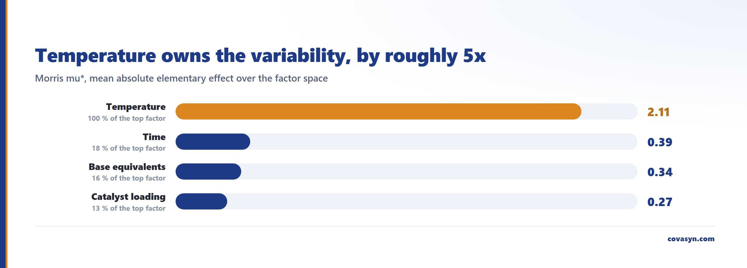
covaopt_robustness ran Morris screening across the four factors:

Factor	Morris mu*	Relative to top
Temperature	2.11	100 %
Time	0.39	18 %
Base equivalents	0.34	16 %
Catalyst loading	0.27	13 %

That is not a close call. Temperature carries roughly five times the elementary effect of the next factor. Three parameters sit in a band so tight that ranking among them is not meaningful at this sample size, which is itself a useful finding: do not spend a control argument distinguishing time from base.

Temperature carries roughly five times the elementary effect of the next factor, so it is the parameter that earns the tight control budget. Source: Computed with covaopt_robustness (Morris screening) on the representative 30-run Pd-catalysed coupling dataset described in this article.

Step 2: get a second opinion from a different method

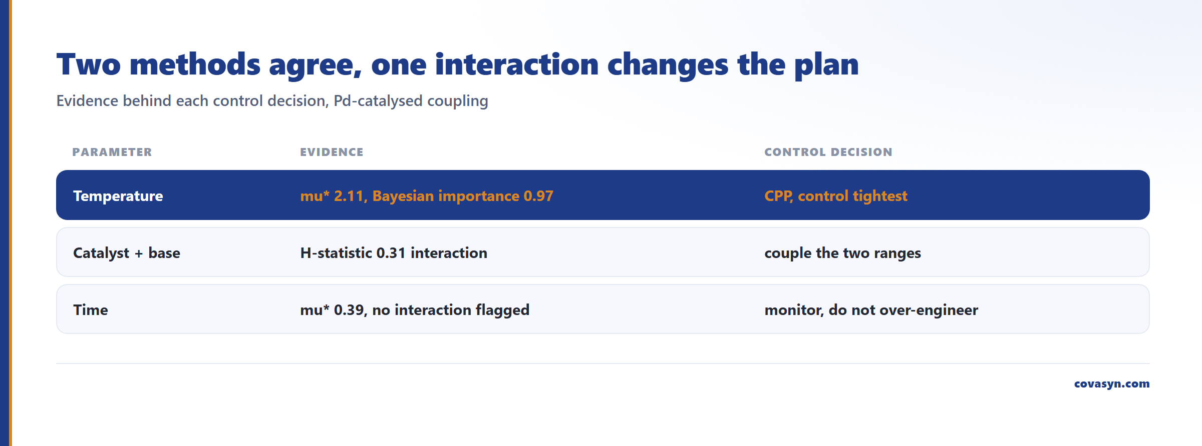
A single sensitivity run is one method's opinion. Bayesian parameter-importance, computed from the optimisation posterior rather than from elementary effects, assigned temperature 0.97 of the total importance. Two methods with different mathematical machinery landing on the same factor is the evidence you want before you write "temperature is the CPP" into a control strategy.

When two methods disagree, that is also informative and usually points at model misspecification or a factor whose range in your data is too narrow to move the response.

Step 3: find the interaction the ranking hides

Ranking is a one-dimensional view. covaopt_explainability computed Friedman's H-statistic and surfaced a catalyst x base interaction of 0.31. Neither factor is individually important by Morris mu*, but together they are not independent. One-factor-at-a-time screening cannot see this by construction, and a main-effects table would have told you to ignore both.

Catalyst and base each look non-critical alone, but their H-statistic 0.31 interaction means their acceptable ranges are conditional and belong in the design space together. Source: Morris mu and Bayesian parameter importance from covaopt_robustness, Friedman H-statistic from covaopt_explainability, on the 30-run Pd-catalysed coupling dataset in this article.

Practically: if you widen the catalyst range, the acceptable base range changes. Your proven acceptable range for one is conditional on the other, and that belongs in the design space description rather than in two separate ranges.

Step 4: propagate the noise you actually have

Ranking tells you what matters. It does not tell you whether your current control is good enough. covaopt_robustness propagated normal operating variation through the fitted models at the recommended setpoint using Monte Carlo over 2,000 draws and returned a 0.0 CQA-failure probability.

Read that carefully. Zero failures were observed in 2,000 draws; that is not the same as failure being impossible. The rule of three puts the upper 95 % bound at roughly 3/2000, about 0.15 %. And it is conditional on the noise distribution assumed per factor. If your real temperature control is worse than assumed, the number moves.

What this changes in the control strategy

The output of this workflow is a defensible allocation, not a report:

1. Temperature: classify as CPP, control tightest. Two independent methods agree, mu* dominates by 5x. This is where the PAT probe and the tightened jacket control go. 2. Catalyst and base: control as a pair. The H-statistic 0.31 interaction means their ranges are coupled. Define them jointly in the design space, not as independent PARs. 3. Time: monitor, do not over-engineer. mu* 0.39, no interaction flagged. A wider operating range is likely defensible if the confirmation runs support it.

For ICH Q8/Q11 purposes this is the evidence a criticality assessment is supposed to rest on: global sensitivity over the whole factor space plus quantified uncertainty, rather than a main-effects plot from a screening design read at nominal conditions.

Honest limits

Sensitivity is bounded by your factor ranges. Morris mu* is the effect *within the range you specified*. Narrow the temperature range and temperature stops looking critical. It never was a property of the parameter alone.
A surrogate model sits underneath. Morris and Sobol on a fitted model inherit that model's errors. In this session the underlying yield model reached cross-validated Q² = 0.80 (ridge poly-2) and purity Q² = 0.72 (random forest) from covaopt_train_models. Below roughly Q² 0.5 the sensitivity ranking is not worth acting on.
Correlated factors break the attribution. If temperature and time were varied together in your historical data, no method can cleanly separate them. Designed experiments can; historical batch records often cannot.
Unmeasured factors do not appear. Raw material lot, humidity, operator, and equipment train are invisible if they are not columns in the dataset. A factor ranking is silent about what you did not record.
0.0 failure probability is a simulation result. It is not a validated capability claim and it is not a substitute for confirmation runs at the edges of the proposed range.
This is 30 runs. The ranking between time, base and catalyst (0.39 / 0.34 / 0.27) is inside the noise you would expect at this n. Treat the top of the list as the finding, not the ordering of the tail.
CovaSyn is decision support and triage. It tells you where to spend experimental effort. It does not replace validated wet-lab confirmation or generate a filing.

Frequently asked questions

What is the difference between Morris and Sobol sensitivity analysis?

Morris screening computes elementary effects at many random points and returns mu*, a mean absolute effect used to rank factors cheaply. Sobol decomposes output variance and returns the exact fraction each factor owns, alone (first-order) and with all its interactions (total-order). Morris is a screening tool costing tens to hundreds of evaluations; Sobol is a quantification tool typically costing thousands. Standard practice is Morris first, Sobol on the survivors.

Can I use SHAP to identify critical process parameters?

SHAP explains the fitted model, not the process. It attributes each prediction to input features and is excellent for interrogating whether a model learned something chemically sensible. But if two parameters are correlated in your historical data, SHAP will distribute credit according to what the model used, which need not match causal process influence. Use SHAP to audit the model, and Morris or Sobol on a sampled factor space to classify CPPs.

How many runs do I need for a meaningful sensitivity analysis?

Sensitivity analysis is run on a fitted model, so the requirement is a model good enough to trust. A practical threshold is cross-validated Q² above about 0.5, with 0.7 or better preferred. The CovaOPT example used 30 runs and reached Q² 0.80 for yield. Below that, the ranking reflects model error rather than process behaviour, and the correct action is more experiments rather than more analysis.

What does Morris mu* actually mean?

mu* is the mean of the absolute elementary effects: the average size of the response change when that factor is stepped, sampled across many random starting points in the factor space. It is a ranking statistic, not a percentage. A mu* of 2.11 for temperature against 0.39 for time means temperature moves the response roughly five times as much on average, in the units of the response, over the ranges you defined.

Does a low sensitivity score mean a parameter is not critical?

Not on its own. Low sensitivity means low influence within the range you tested, which is a statement about your range as much as about the parameter. Also check the interaction terms: in the worked example, catalyst and base both scored low individually (mu* 0.27 and 0.34) but showed a real catalyst x base interaction with H-statistic 0.31. A parameter can be non-critical alone and critical in combination.

How does this support an ICH Q8 criticality assessment?

It supplies global sensitivity over the whole multivariate factor space plus quantified uncertainty at the proposed setpoint, which is what a criticality argument needs to be more than an opinion. It does not by itself constitute the assessment. You still need the risk assessment, confirmation runs at the range edges, and a control strategy that ties each classified CPP to a specific control.