Split-Plot Designs for Hard-to-Change Factors

Your DoE software hands you a 16-run randomised design and the first three rows tell you to run 70 C, then 110 C, then 70 C again. On paper that is one column of numbers. In the lab it is three thermal cycles on a jacketed reactor, each an hour of ramp and equilibration, and by run 6 the chemist has quietly sorted the sheet by temperature. That reordering is not sloppiness. It is a split-plot design, and if you analyse the data as if it were still fully randomised your p-values are wrong.

Every number below is output from the CovaDOE MCP tools (covadoe_create_design and covadoe_analyze), generated on 2026-07-15.

What makes a factor hard to change

A factor is hard to change when resetting it costs materially more than running the experiment itself. In practice:

• Reactor or oven temperature - ramp, soak, re-equilibrate.
• Batch of raw material or catalyst lot - you get one drum, you use it up.
• Column or instrument configuration - swapping an HPLC column and re-equilibrating.
• Operator, shift or day - you cannot randomise Tuesday.

Everything else - catalyst loading, base equivalents, reaction time, dilution - is easy to change at no real cost per run.

Complete randomisation assumes every run is an independent reset of the whole system. When temperature is hard to change, that assumption is false, and pretending otherwise is the most common silent error in industrial DoE.

The whole-plot / sub-plot structure

Declare the hard-to-change factor and the design reorganises itself. Here is covadoe_create_design with design_type="full_factorial_2k", four factors, and hard_to_change=["Temperature"]:

The tool returns 16 runs and a new column, WholePlot. Its design_info field reads verbatim:

"split_plot": {"hard_to_change": ["Temperature"],
               "n_whole_plots": 2,
               "whole_plot_sizes": [8, 8]}

Runs 1 to 8 sit at 70 C, runs 9 to 16 at 110 C. Two thermal setups instead of an expected eight or nine under full randomisation. The vocabulary:

• Whole plot - one setting of the hard-to-change factor, held while several runs are executed. Here, one temperature campaign.
• Sub plot - the individual runs inside a whole plot, where the easy factors are randomised freely.
• Restricted randomisation - you randomise the order of whole plots, and independently the order of runs within each whole plot. You do not randomise across them.

One trap worth knowing

Setting n_replicates=2 on a two-level hard-to-change factor does not buy you more whole plots. Re-running the same design with three factors and two replicates still returned "n_whole_plots": 2, "whole_plot_sizes": [8, 8]. The tool groups by distinct hard-to-change setting, so replicate runs land inside the existing plots. If you want independent whole-plot replication - and for a proper whole-plot error term you do - you have to physically tear the setup down and rebuild it, and assign the WholePlot labels yourself.

The analysis consequence, with real numbers

This is where it matters. A split-plot experiment has two error terms, not one:

• Whole-plot error - variation between reactor setups. Reactor cleaning, thermocouple placement, a slightly different ramp profile.
• Sub-plot error - variation between runs inside one setup. Usually much smaller, because the big sources of variation are held fixed.

The hard-to-change factor is tested against the whole-plot error. The easy factors and their interactions are tested against the sub-plot error.

Worked example: the same reactor system, four whole plots (two at 70 C, two at 110 C, each torn down and rebuilt), four sub-plot runs each. covadoe_analyze picks up the WholePlot column automatically and returns both fits side by side. Per-run yields here were simulated from a known model with a whole-plot offset, standing in for lab measurements; every statistic below is a genuine tool computation on that data.

Standard OLS (the `WholePlot` column ignored):

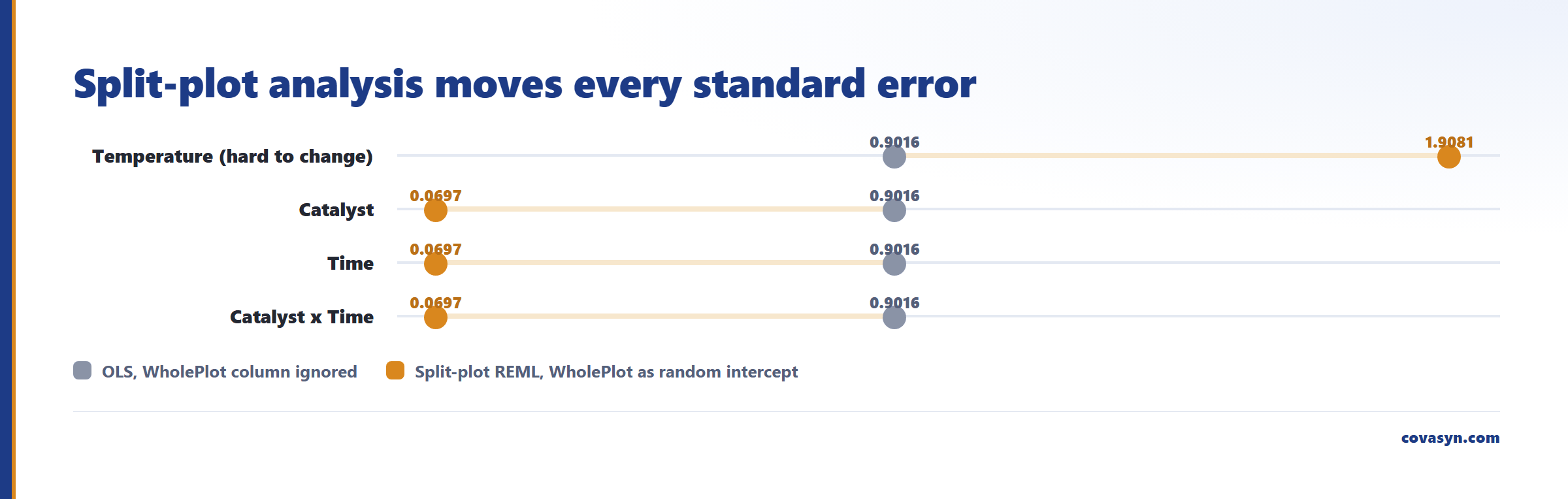
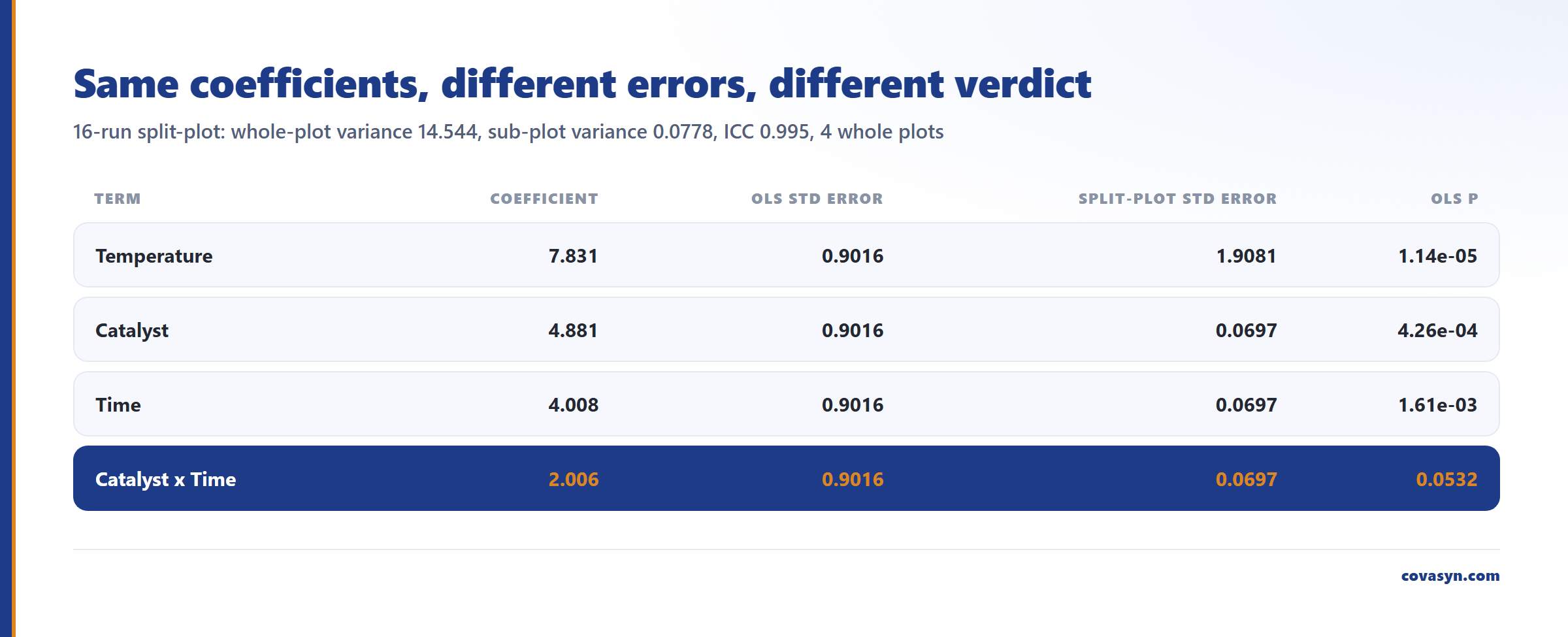
R-squared 0.9350, residual MS 13.006 on 9 df. Every term gets the same standard error, because OLS assumes one pooled error. The Catalyst x Time interaction lands at p = 0.0532 and you write it off.

Split-plot fit (`WholePlot` as a random intercept, REML):

Variance components from the tool: whole-plot variance 14.544, residual (sub-plot) variance 0.0778, ICC 0.995, 4 whole plots.

Read the two tables against each other:

1. The coefficients are identical. Split-plot analysis does not change your effect estimates here. It changes what you are allowed to say about them. 2. The hard-to-change factor gets a bigger standard error. Temperature goes from 0.9016 to 1.9081, a factor of 2.1. You have four thermal setups, not sixteen independent runs, so the temperature effect rests on far less information than the run count suggests. OLS was overstating your confidence in the one factor you probably care about most. 3. The easy factors get a much smaller standard error. Catalyst goes from 0.9016 to 0.0697. Holding temperature fixed inside a plot removes the setup-to-setup noise from the within-plot comparisons, and the sub-plot effects are measured far more sharply. The interaction that OLS called borderline at p = 0.0532 is real. 4. ICC 0.995 says almost all the variance is between plots. That is the diagnostic. If ICC is near zero, restricted randomisation cost you nothing. Near one, and the OLS analysis is badly misleading.

There is a fourth number worth flagging. The OLS lack-of-fit test reported ss_pure_error = 117.057 on 8 df with a lack-of-fit p of 1.0 - a clean bill of health. That "pure error" is largely whole-plot variation misfiled as replicate noise. A split-plot design analysed as a CRD can look like a well-fitting model while the error structure is wrong.

Practical rules

• Declare hard-to-change factors before you generate the design, not after the data is in. hard_to_change changes the run layout, not just the analysis.
• Aim for at least four whole plots, more if the hard-to-change factor is your main question. Two whole plots leaves zero degrees of freedom for whole-plot error and no honest test of the hard-to-change effect.
• Whole-plot replication means a genuine teardown and rebuild. Two runs in the same reactor charge are sub-plot replicates, whatever the sheet says.
• Keep the WholePlot column all the way to analysis. covadoe_analyze looks for it by name; drop it and you silently get the OLS answer.
• If your chemist re-sorted an existing randomised sheet by temperature, you already ran a split-plot experiment. Reconstruct the whole-plot labels from the lab notebook and re-analyse.

What this does not tell you

• It does not recover power for the hard-to-change factor. The split-plot analysis reports your temperature effect honestly; it does not make it better. If temperature is the primary question, buy more whole plots, not more sub-plot runs.
• The sub-plot p-values in the example are extreme by construction. The simulated sub-plot noise was small (residual variance 0.0778), so the REML standard errors are correspondingly tiny. Take the direction of the shift as the lesson, not the magnitude. Real assay noise will be larger.
• Four whole plots is a thin basis for a variance component. The 14.544 whole-plot variance is estimated from four setups. Treat it as an order of magnitude, not a validated number.
• A split-plot layout does not fix a bad factor range. If your temperature window is narrower than your process noise, no error structure rescues the experiment. And this is design and analysis support, not a filing: any design space or NOR you derive still needs confirmation runs on the real equipment.

Frequently asked questions

Related reading

• Central composite vs Box-Behnken designs
• Definitive screening design: a real 13-run example
• Power analysis before you run the experiment
• ICH Q8 design space, NOR and PAR explained

You can generate a split-plot layout and run the two-error-term analysis yourself on the CovaSyn free tier.