Guide8 min readJuly 15, 2026

Response Surface Methodology, End to End

A response surface methodology tutorial with real CovaDOE output: 18-run CCD, quadratic fit R2 0.9988, optimum with CIs, design space and residual.

Oliver Kraft

CovaSyn

Response Surface Methodology, End to End

Screening told you which factors matter. It did not tell you where to set them. Response surface methodology (RSM) is the second half of the job: fit a curved model over the factors you kept, find the optimum, and put an operating region around it that survives normal process variation.

This article walks the sequence on one three-factor catalytic step using the CovaDOE tools. Every number is verbatim tool output; the caveat on where those numbers come from is in the honest-limits section.

The five steps, in order

1. Build a design that can estimate curvature (covadoe_create_design). 2. Run it and fit the quadratic model (covadoe_fit_rsm). 3. Check the residuals before you believe the model (covadoe_residual_diagnostics). 4. Locate the optimum and put an interval on it (covadoe_find_optimum, covadoe_predict). 5. Turn the point into a region (covadoe_design_space).

Steps 3 and 5 are the ones people skip. Step 3 is where you find out the model is lying; step 5 is where the filing value is.

Step 1: a design that can see curvature

A two-level screening design cannot fit a quadratic term; you need at least three levels per factor. This example uses a central composite design (CCD) on:

Temperature: 70 to 110 C
Catalyst loading: 1 to 6 mol%
Time: 4 to 14 h

covadoe_create_design with design_type="central_composite" and n_center_points=4 returned 18 runs: 8 factorial corners, 6 axial (star) points, 4 centre points, rotatable at alpha = 2.236.

Two practical notes. The 4 replicated centre points give you pure error, and pure error is what lets you test lack of fit later - do not trim them to save runs. And check the axial points in real units first: at alpha = 2.236 they sit outside the stated range, which is fine for temperature and fatal for a factor with a hard floor at zero. If your axials come back negative, use Box-Behnken instead.

Step 2: fit the quadratic model

With the 18 responses in hand, covadoe_fit_rsm fitted the full quadratic model - 3 linear, 3 quadratic and 3 two-factor interaction terms plus intercept:

Metric	Value
R2	0.9988
Adjusted R2	0.9974
Term significance	all terms p < 1e-4
Model form	full quadratic, 3 factors

Read those two R2 values as a pair, always. R2 only goes up when you add terms; adjusted R2 penalises terms that do not earn their place. Here the gap is 0.0014, so the model is not padded. A large gap - say R2 0.98 against adjusted 0.89 - means you are fitting noise with interaction terms, and you should drop the ones that fail significance and refit.

An R2 of 0.9988 is high by lab standards. On real assay data with 2 to 3 percent repeatability, expect 0.90 to 0.97, and be suspicious of anything above 0.999 you did not simulate yourself.

Step 3: check the residuals before you believe any of it

This separates a model you can defend from a number you copied out of a report. covadoe_residual_diagnostics on the same fit returned:

Shapiro-Wilk p = 0.036 on the residuals. Below 0.05, so the normality assumption is formally rejected at the 5 percent level.
Cook's distance 0.277 at run 9, flagged as the most influential run.

Neither invalidates the model, and neither should be ignored.

Shapiro-Wilk p = 0.036 with n = 18.

Normality tests on 18 residuals have low power, so a marginal p is weak evidence either way. It usually points at one or two outlying runs, not a genuinely skewed error distribution. Plot residuals against fitted values: a funnel shape means non-constant variance, which is a real problem and is usually fixed by a log or square-root transform of the response. A marginal Shapiro p with a clean residual plot is something you note and move past.

Cook's D 0.277 at run 9.

Cook's distance measures how much the fitted surface moves if you delete that run. Run 9 is an axial point, and axial points have high leverage by construction - furthest from the centre, so they pull hardest on the quadratic terms. A common threshold is 4/n, here 0.222, so 0.277 is over it but not dramatically. Do not delete the run. Go back to the notebook and ask whether anything about it was unusual: a different reagent lot, a manual temperature hold, a late sample. If nothing was, keep it and say so.

Never delete a run for being statistically inconvenient - only for a documented physical cause, recorded. If you refit without it, report both fits.

Step 4: the optimum, with error bars

covadoe_find_optimum on the fitted surface returned, inside the design bounds:

Temperature 91.2 C
Catalyst 3.76 mol%
Time 9.7 h
Predicted yield 93.5 percent

covadoe_predict at that setting gave:

Interval	Range
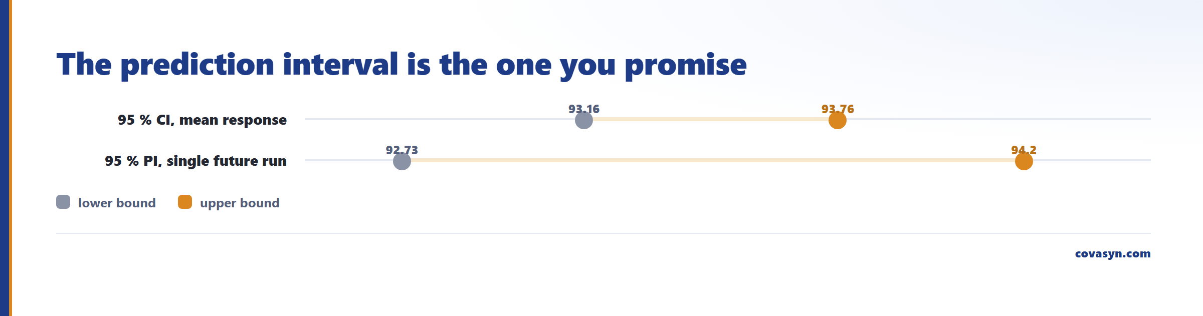
95 percent confidence interval (mean response)	93.16 to 93.76 percent
95 percent prediction interval (single future run)	92.73 to 94.20 percent

People get this distinction backwards. The confidence interval is where the true average yield at that setpoint sits. The prediction interval is where your next single batch lands; it is always wider because it carries run-to-run noise on top of parameter uncertainty. Promising a colleague a yield for one confirmation run means quoting 92.73 to 94.20, not the confidence interval.

At the RSM optimum the confidence interval covers the true mean yield; the wider prediction interval, 92.73 to 94.20 percent, is where a single confirmation batch lands. Source: Computed with covadoe_predict at the covadoe_find_optimum setpoint (91.2 C, 3.76 mol%, 9.7 h, predicted 93.5 % yield) on the 18-run CCD in this article.

Note also that the optimum sits at 91.2 C well inside the 70 to 110 C range. An optimum that lands on a boundary is not an optimum; it means the range was truncated too early and the surface is still climbing. Widen and rerun.

Step 5: from a point to a design space

A single setpoint is not a manufacturable process. covadoe_design_space propagates the model plus its uncertainty through 10,000 Monte Carlo samples and returns the region where the response stays inside spec.

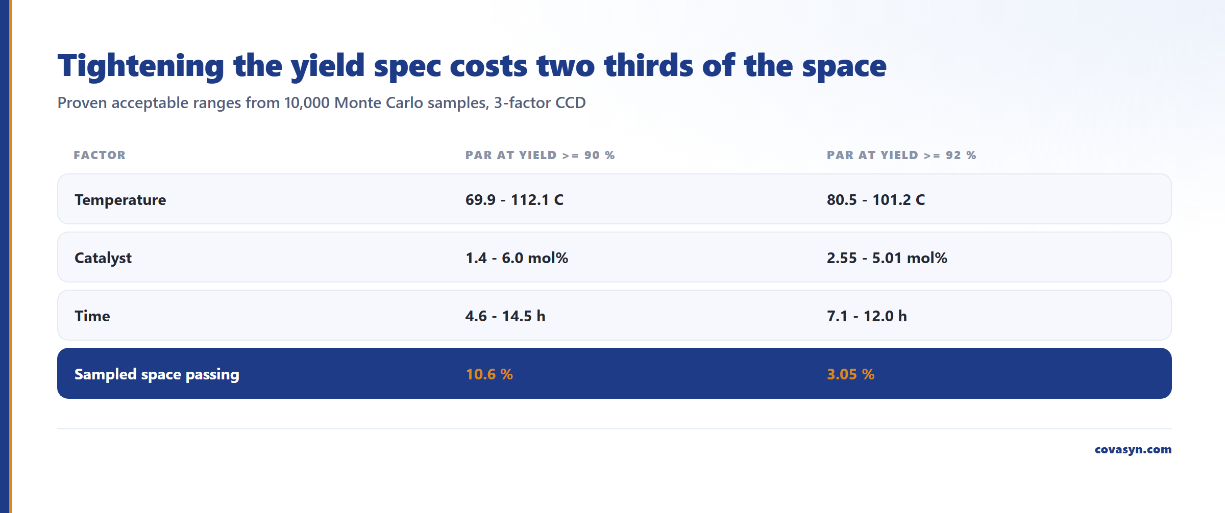
At a specification of yield >= 90 percent:

Factor	Proven acceptable range
Temperature	69.9 to 112.1 C
Catalyst	1.4 to 6.0 mol%
Time	4.6 to 14.5 h
Fraction of sampled space passing	10.6 percent

Tighten the spec to >= 92 percent and the window contracts to 80.5 to 101.2 C, 2.55 to 5.01 mol%, 7.1 to 12.0 h, with only 3.05 percent of the sampled space passing.

That pair of numbers prices the specification. Moving from 90 to 92 percent yield costs roughly two thirds of your operating room and shrinks the temperature window from 42 degrees to 21. Have that conversation with the process owner before the limit goes into a control strategy, not after.

The design space prices the specification: two extra yield points cut the temperature window from 42 degrees to 21 and the passing fraction from 10.6 to 3.05 percent. Source: Computed with covadoe_design_space over 10,000 Monte Carlo samples on the 18-run central composite design in this article; the per-run yields feeding the fit were simulated from a quadratic surface with noise.

One tooling gotcha: covadoe_design_space expects spec_lower and spec_upper. Pass lower/upper by mistake and it silently returns a pass probability of 1.0 and the full factor range. A design space that comes back suspiciously wide with a probability of exactly 1.0 is a keyword bug, not a robust process.

What RSM does not tell you

The model is only valid inside the design region. A quadratic fitted between 70 and 110 C says nothing about 130 C. Polynomial extrapolation is not just uncertain, it is often confidently wrong in the opposite direction.
A high R2 is not a correct model. A quadratic can fit a sigmoid well over a narrow window and fail badly just outside it. R2 measures fit to the runs you did, not mechanism.
Design space output is model-based, not measured. The Monte Carlo samples propagate the fitted model. They cannot know about a phase change, a solubility limit or a catalyst deactivation the design never sampled. Edge confirmation runs are not optional.
This example is partly simulated. The 18-run CCD is a genuine design and every statistic quoted - R2, optimum, intervals, design-space ranges, diagnostics - is a real CovaDOE computation. The per-run yields feeding it were simulated from a quadratic surface with noise, standing in for lab measurements. That is why the R2 is unusually high. Treat this as a demonstration of the workflow, not a benchmark of achievable yield.
This is decision support, not a filing. CovaDOE output helps you design, analyse and argue. It does not replace wet-lab confirmation, a validated statistics package or your own regulatory review.

Frequently asked questions

What is response surface methodology?

Response surface methodology is a design-of-experiments approach for modelling a curved relationship between process factors and a response. You run a three-level design such as a central composite or Box-Behnken, fit a quadratic model with linear, squared and interaction terms, then use that model to locate an optimum and define an operating region. It follows screening, which identifies which factors matter.

How many runs does a response surface study need?

A full quadratic model in 3 factors has 10 parameters, so you need more than 10 runs plus replicates for pure error. A 3-factor central composite design with 4 centre points came back from covadoe_create_design as 18 runs: 8 factorial corners, 6 axial points and 4 centre points. Box-Behnken needs 16 with the same centre replication. Run counts grow quickly beyond 4 factors.

What is a good R2 for a response surface model?

Look at R2 and adjusted R2 together rather than at R2 alone. In the CovaDOE example, covadoe_fit_rsm returned R2 0.9988 with adjusted R2 0.9974, a gap of 0.0014, meaning no term was padding the fit. On real assay data with a few percent repeatability, 0.90 to 0.97 is a realistic target. A wide R2 to adjusted-R2 gap means you are fitting noise.

What is the difference between a confidence interval and a prediction interval in RSM?

The confidence interval covers the true mean response at a setpoint; the prediction interval covers a single future run and is always wider because it adds run-to-run noise. At the optimum in this example, covadoe_predict returned a 95 percent confidence interval of 93.16 to 93.76 percent and a prediction interval of 92.73 to 94.20 percent. Quote the prediction interval for a confirmation batch.

What does Cook's distance flag in a DoE model?

Cook's distance measures how much the fitted surface would move if one run were removed. covadoe_residual_diagnostics flagged run 9 at Cook's D 0.277 against a common 4/n threshold of 0.222 for 18 runs. In a central composite design, high values often land on axial points because they have the highest leverage. Investigate the run physically; do not delete it for being statistically inconvenient.

Should I worry about a failed normality test on my residuals?

A marginal result deserves a look, not a panic. Shapiro-Wilk returned p = 0.036 on the 18 residuals here, formally rejecting normality at 5 percent, but the test has low power at that sample size. Plot residuals against fitted values first: a funnel shape indicates non-constant variance and calls for a response transform, while a clean plot with one outlier usually points to a single unusual run.