Use Case8 min readJuly 15, 2026

QbD Process Development: Screen, RSM, ML in One Run

A QbD process development workflow end to end: DoE screen, response surface, ML model on one 29-run Pd coupling, with every number a real CovaDOE and.

Oliver Kraft

CovaSyn

QbD Process Development: Screen, RSM, ML in One Run

Most process development runs as three disconnected exercises. Someone screens factors in a spreadsheet, someone else fits a response surface months later, and a data scientist trains a model on whatever rows survived. Nobody checks whether the three agree. This article walks one Pd cross-coupling through all three stages on a single 29-run dataset, and shows what the agreement between them is worth.

The workflow in one line

Screen to find out what matters. Model the survivors to find the optimum. Then model the whole dataset a second way, with a different method, to see whether the answer holds.

The three stages are not redundant. Screening is cheap and answers a ranking question. Response surface modelling is expensive per factor and answers a location question. A cross-validated machine-learning model answers a robustness question: does the optimum survive a method that makes none of the polynomial assumptions the RSM makes.

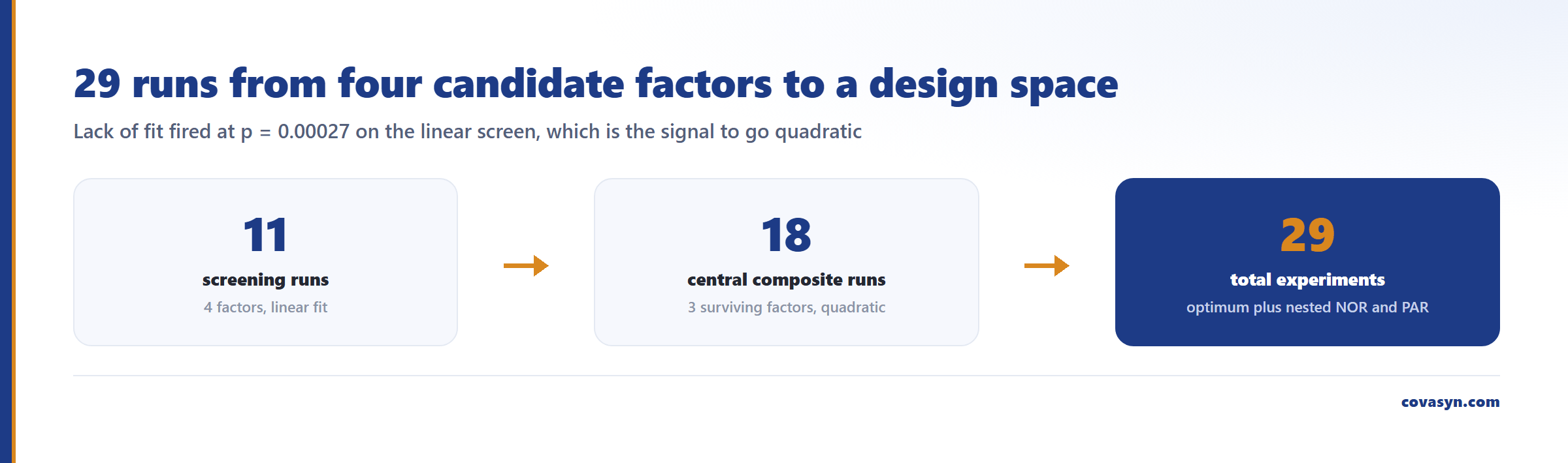
Total experimental cost in the example below: 29 runs. That is the whole story from "we have four candidate factors" to "here is a control strategy with a nested NOR and PAR".

Stage 1: screen, and let the design tell you when to stop

Four candidate factors: temperature, catalyst loading, reaction time, base equivalents. An 11-run screening design, built with covadoe_create_design and fitted linear with covadoe_fit_rsm.

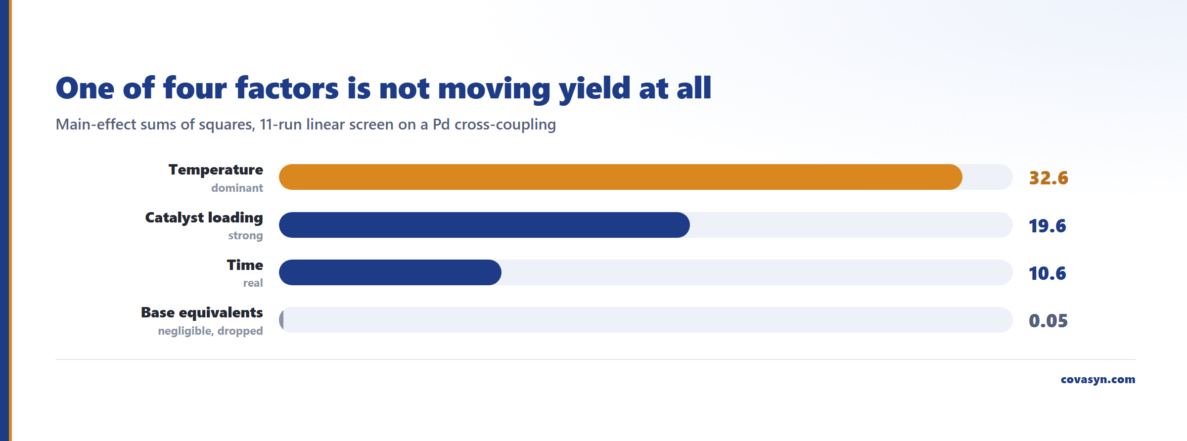
The main-effect sums of squares came back:

Factor	Main-effect SS	Read
Temperature	32.6	dominant
Catalyst loading	19.6	strong
Time	10.6	real
Base equivalents	0.05	negligible

Base equivalents contributes 0.05 against a temperature effect of 32.6, roughly three orders of magnitude smaller. That factor is not driving yield inside the ranges tested. Drop it, and you have taken a four-factor problem down to three before spending a single run on a response surface. That is where the savings in DoE actually come from: not from the screen itself, but from what the screen lets you not do next.

Base equivalents contributes 0.05 against temperature's 32.6, so it is dropped before the response surface stage. That is where the savings in DoE actually come from. The Pd-coupling inputs are illustrative rather than a specific customer campaign; every statistic quoted is a genuine tool computation on that dataset. Source: Computed with covadoe_create_design and covadoe_fit_rsm on the 11-run screening stage of the 29-run Pd coupling dataset described in this article.

The second output matters more than the ranking. The lack-of-fit test fired at p = 0.00027. The linear model cannot describe this data. The centre points sit well above the plane through the corners, which is the classic signature of curvature: there is an interior maximum somewhere between the corner settings.

That is a decision, not a plot. A significant lack of fit at the screening stage means stop screening. More linear runs will not help. Go quadratic.

Stage 2: response surface on the survivors

Three factors, an 18-run central composite design, quadratic fit via covadoe_fit_rsm: R-squared 0.922, all quadratic terms significant and negative.

Negative quadratic terms in every factor is the condition for a true interior maximum rather than an edge optimum. If a quadratic term had come back positive or non-significant, the surface would be a ridge or a plane and the "optimum" would just be the corner of your experimental box.

covadoe_find_optimum located the stationary point:

84.7 C, 1.39 mol% catalyst, 11.1 h
Predicted yield 93.63%, 95% confidence interval 92.98 to 94.28%

Quote that interval when someone asks how sure you are. It is roughly plus or minus 0.65 percentage points on the mean response, which is tight enough to design a control strategy around and loose enough that you should not argue about the third decimal place.

covadoe_design_space then wrapped a PAR around the optimum at a yield acceptance criterion of >= 92%. That is the region you would carry into an ICH Q8 design space discussion.

Cost so far: 11 + 18 = 29 runs, and you have a defensible optimum with an interval on it.

The screen is what makes this affordable: dropping a negligible factor removes runs from the expensive quadratic design, not from the cheap linear one. Source: Run counts and lack-of-fit p value from covadoe_create_design and covadoe_fit_rsm on the Pd coupling dataset described in this article.

Stage 3: a second opinion from a different method

Now feed all 29 runs, screen and CCD together, to covaopt_train_models. This fits multiple model families with cross-validation and selects on out-of-fold performance, so it is not the same mathematics as the RSM and it does not assume a quadratic form.

Results:

Response	Cross-validated Q-squared	Gate
Yield	0.89	passes, use for optimization
Purity	0.53	fails, monitor only

Two things to take from that table. First, yield at Q-squared 0.89 is a model you can optimize against. Second, purity at 0.53 is not, and the tool says so rather than handing you a number to steer by. In this dataset purity sits near its ceiling with very little variance, so there is almost nothing for a model to learn. A near-ceiling response with low variance is a common and honest reason for a weak model. The correct action is to keep purity as a monitored attribute and not to put it in the objective function.

Three checks on the yield model:

1. Factor ranking reproduces the screen. ML feature importance put temperature at 0.61, ahead of catalyst loading, ahead of time. Same order as the screening sums of squares, from a completely different estimator. 2. Optimum reproduces the RSM. The ML setpoint landed at 85.2 C, 1.40 mol%, 10.9 h predicting 93.4% yield, against the RSM's 84.7 C / 1.39 mol% / 11.1 h predicting 93.63%. Half a degree, 0.01 mol%, 0.2 h apart. 3. The ranges nest. covaopt_design_space returned a NOR and PAR that sit inside the RSM design space rather than straddling its edge. A control strategy where the model-derived operating band contradicts the RSM band is a strategy you have to defend twice.

covaopt_process_capability then ran the SPC view on the same data: the process is in statistical control with 0.0% out-of-spec points. Note what this is and is not: it is control-chart evidence, not a capability index. This deployment did not return a numeric Cpk because the specification limits were not supplied to it, and we are not going to quote one that was not computed.

Why convergence is the deliverable

Three methods, one dataset, one answer:

Stage	Tool	Top factor	Optimum	Predicted yield
Screen (11 runs)	`covadoe_create_design`, `covadoe_fit_rsm`	temperature (SS 32.6)	curvature detected, p = 0.00027	-
RSM (18 runs)	`covadoe_find_optimum`	-	84.7 C / 1.39 mol% / 11.1 h	93.63% (CI 92.98-94.28)
ML (all 29 runs)	`covaopt_train_models`	temperature (0.61)	85.2 C / 1.40 mol% / 10.9 h	93.4%

If the RSM optimum and the ML optimum had disagreed by ten degrees, you would have learned something important: either the quadratic form is wrong, or the ML model is fitting noise, or there is structure in the data one of them is missing. Disagreement between methods is a diagnostic. Agreement is the closest thing you get to internal validation without spending more runs.

What this workflow does not tell you

It is not confirmation. All three stages read the same 29 experiments. Agreement rules out method artefacts; it does not rule out a systematic error in the data itself. You still run confirmation batches at the proposed setpoint.
It does not extrapolate. Every range quoted is inside the experimental envelope. The model says nothing defensible about 120 C if you never ran above 100 C.
Purity is unmodelled here. Q-squared 0.53 means the purity surface is not characterised. If purity is a CQA, it needs its own study with runs that actually move it.
No capability index. 0.0% out-of-spec is in-control evidence from SPC. It is not a Cpk or Ppk claim, and it is not a validation result.
This dataset is representative. The Pd-coupling inputs are illustrative rather than a specific customer campaign. Every statistic quoted above, including the sums of squares, the lack-of-fit p value, R-squared, Q-squared, the optima and the intervals, is a genuine tool computation on that data, not an estimate written into a slide.

Frequently asked questions

How many experiments does a QbD process development workflow need?

In the worked example above, 29 runs took a four-factor Pd coupling from an unscreened problem to a characterised optimum with a nested operating range: an 11-run screening design, then an 18-run central composite on the three factors that survived. The screen is what makes this affordable, because dropping one negligible factor before the response surface stage removes runs from the expensive design, not the cheap one.

When should you stop screening and switch to a response surface design?

When the lack-of-fit test on the linear screening model becomes significant. In the example, covadoe_fit_rsm returned lack-of-fit p = 0.00027, meaning the centre points sat far above the plane through the corner runs. That is curvature, and no amount of additional linear runs will resolve it. Drop the negligible factors and augment to a quadratic design.

Does machine learning replace design of experiments in process development?

No. In this example the ML model was trained on the DoE runs and could not have existed without them. Its value was corroboration: cross-validated yield Q-squared 0.89, a feature ranking that reproduced the screening order with temperature at 0.61, and a setpoint 0.5 C from the RSM optimum. ML answers whether the answer survives a different method, not whether you can skip the experiments.

What does a low Q-squared on one response mean?

It means that response is not modelled well enough to optimize against and should be monitored instead. In the worked example, purity returned Q-squared 0.53 because it sat near its ceiling with very little run-to-run variance, so there was almost no signal to learn. The honest action is to exclude it from the objective function and keep it as a monitored attribute.

Why should the ML operating range sit inside the RSM design space?

Because a control strategy with two contradictory acceptable regions has to be defended twice. In the example, covaopt_design_space returned NOR and PAR ranges nested inside the response-surface design space, so the model-based and the RSM-based views agree on where the process may run. If they had straddled, that mismatch is the first thing to resolve before proposing anything.