

You have six months of 40 °C accelerated data, three months of 25 °C long-term data, and a project team that wants a shelf life number now. The regulatory answer is that shelf life comes from long-term data. The practical answer is that you still have to make a decision today, and your accelerated arm already contains most of the information you need. This article covers how the two methods work, what ICH Q1E actually permits you to extrapolate, and where the whole approach breaks down.
The two numbers you are trying to reconcile
There are two independent routes to a 25 °C shelf life, and a good stability package uses both.
Route 1: kinetics (Arrhenius).
Extract a degradation rate at each storage temperature, regress ln(k) against 1/T, and use the fitted activation energy to project the rate at 25 °C. Then solve for the time at which the projected assay hits your specification limit. This route is fast: it works as soon as the accelerated arm has enough timepoints to give a reliable rate.
Route 2: ICH Q1E regression.
Regress the long-term 25 °C data against time, take the 95% one-sided confidence limit of the mean curve, and read off where that limit crosses the acceptance criterion. This is the route that goes in the dossier. It is slower, because it is limited by how long the long-term arm has been running.
Route 1 is a prediction. Route 2 is the regulatory calculation. If they agree, you have convergent evidence and a defensible position. If they disagree badly, something in your model or your data is wrong, and it is better to find that out at month 6 than at month 24.
What ICH Q1E actually lets you extrapolate
This is the part that gets misremembered most often. Q1E does not let you file an Arrhenius number as your shelf life. It lets you extrapolate the long-term regression by a bounded amount, and it uses the accelerated and intermediate data to decide how much.
| Situation at accelerated (40 °C / 75% RH) | What Q1E allows |
|---|---|
| No significant change over 6 months, long-term data show little change and little variability | Up to 2X the long-term period covered, capped at +12 months, often without formal statistical analysis |
| No significant change at accelerated, but long-term data show change or variability | Up to 2X, capped at +12 months, with statistical analysis backing it |
| Significant change at accelerated, no significant change at intermediate (30 °C) | Reduced extrapolation: roughly 1.5X the long-term period, capped at +6 months |
| Significant change at intermediate as well | No extrapolation. Shelf life is the period covered by long-term data, or shorter |
Two further Q1E specifics worth having in your head: batch poolability is judged with an ANCOVA at the 0.25 significance level (a deliberately permissive threshold, because failing to pool is the conservative outcome), and the shelf life is taken from the 95% one-sided confidence limit rather than the fitted mean line. Check the Appendix A decision trees against your own case before committing to an extrapolation: they branch on drug substance versus drug product and on whether the attribute is expected to increase, decrease or stay flat.
Worked example: a small-molecule drug product
The dataset below is a representative small-molecule drug product stability set: assay as % label claim, arms at 25 °C, 30 °C and 40 °C, specification at 95% LC. The inputs are representative. Every number quoted here comes unchanged from CovaSyn's stability analysis, computed on that data, not a hand-fitted spreadsheet number.
Step 1: fit the temperature dependence.
The Arrhenius fit returns:
- Activation energy Ea = 107.45 kJ/mol
- Q10 = 4.08
- Arrhenius fit R2 = 0.995
A Q10 of 4.08 means roughly a fourfold increase in degradation rate per 10 °C. That single number explains why the accelerated arm is useful: at 40 °C the molecule is degrading about eight times faster than at 25 °C, so six weeks of 40 °C data carries about as much degradation signal as a year at 25 °C. An Ea of 107 kJ/mol sits in the normal range for small-molecule hydrolytic and oxidative degradation, which is a sanity check worth doing: values far outside roughly 50 to 150 kJ/mol usually mean the rate extraction or the mechanism assumption is off.
Step 2: project to the storage condition.
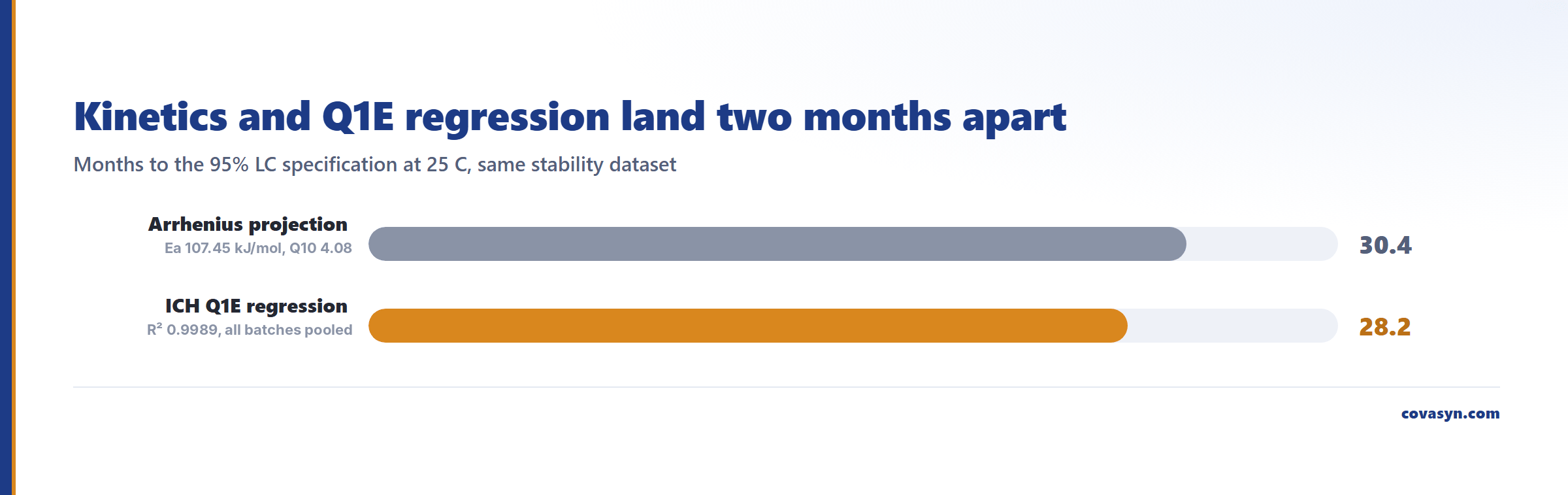
The projection to storage temperature returns 30.4 months to the 95% LC spec at 25 °C, projected from the 40 °C and 30 °C rates through the Arrhenius fit.
Step 3: run the Q1E calculation independently.
The Q1E long-term regression returns 28.2 months, with regression R2 = 0.9989 and a slope p-value of 1.3e-8. The poolability check allows all batches to be pooled, meaning the batches were not statistically distinguishable at the Q1E threshold and were analysed as a single pooled dataset.
Step 4: do not choose the kinetic order by R2.
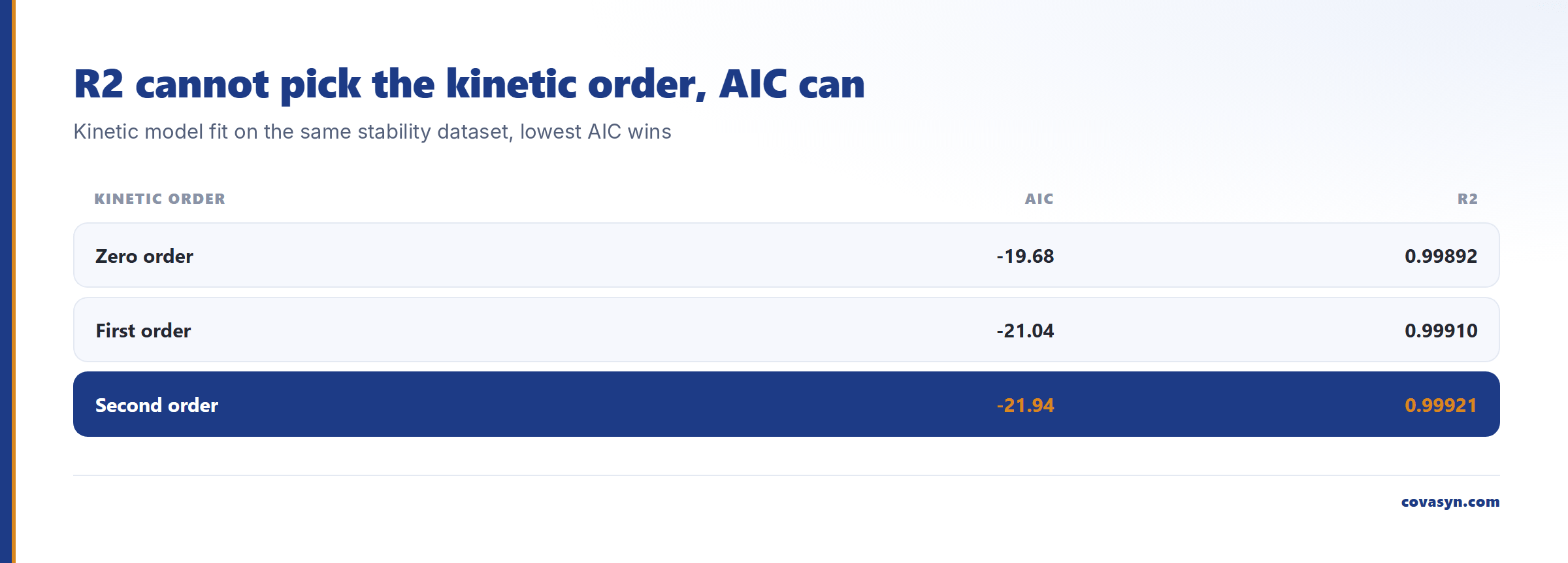
The candidates are practically level at R2 0.99892, 0.99910 and 0.99921, with AIC values of −19.68, −21.04 and −21.94. Differences below about 2 AIC units do not separate models. The data do not distinguish the orders in this range; decide on mechanism and, when in doubt, choose the simpler model. For the Q1E shelf life this hardly matters, because all three are practically linear in the range used.
The reconciliation.
30.4 months from kinetics, 28.2 months from the regression of the long-term data: about two months apart. The regression gives the point where the confidence bound meets the specification. What you may propose is limited by ICH Q1E: at most twice the period covered by long-term data and no more than 12 months beyond it. With 12 months of long-term data that is 24 months, with 3 months only 6. The Arrhenius number supports the decision early; the shelf life in the dossier follows from regression and extrapolation limit.
What these numbers do not tell you
Be blunt about this internally, because reviewers will be.
- Arrhenius assumes one dominant mechanism that does not change with temperature. If 40 °C activates a pathway that is negligible at 25 °C, or if a phase change, melting or moisture-uptake event occurs between the conditions, the extrapolation is invalid no matter how good the R2 is. An R2 of 0.995 on three temperature points is not proof of mechanistic constancy: it is three points.
- 30.4 months is a prediction, not a shelf life. It supports a decision (formulation ranking, packaging choice, go/no-go on a stability protocol). It is not a filing number and our analysis does not make it one.
- Assay is not the only stability-indicating attribute. Shelf life is set by whichever attribute fails first: total degradants, a specified impurity, dissolution, water content, appearance, microbial limits. An assay-based calculation is one input.
- Solid-state and biologic products often violate the assumption outright. Amorphous dispersions, lyophilised products and proteins frequently show non-Arrhenius behaviour. Treat kinetic extrapolation there as hypothesis generation only.
- The statistics do not fix a thin design. Three batches with sparse timepoints will give a wide confidence limit, and the Q1E shelf life comes from the limit, not the mean. Design the study properly; no model recovers information that was never collected.
- Caveat from our own testing: in the run above, the separately reported poolability check and the separate rate extraction could not be verified, and none of their numbers are quoted here. The pooling verdict comes from the poolability check inside the Q1E regression. We would rather say that than quietly present a number we did not verify.
Frequently asked questions
How is shelf life calculated under ICH Q1E?
ICH Q1E calculates shelf life by regressing the long-term stability data against time and finding the point where the 95% one-sided confidence limit of the mean curve intersects the acceptance criterion. Batches are tested for poolability by ANCOVA at the 0.25 significance level; if poolable, all batches are regressed together. The result may then be extrapolated by a bounded amount that depends on the accelerated and intermediate data.
Can I use accelerated data to set shelf life?
Not directly. Accelerated data support extrapolation of the long-term result rather than replacing it. Under ICH Q1E, if there is no significant change at accelerated conditions over six months, you may extrapolate the long-term regression to up to twice the period covered, capped at 12 months beyond it. Arrhenius projections from accelerated data are decision-support during development, not a filing number.
What is Q10 and why does it matter for stability?
Q10 is the factor by which the degradation rate increases per 10 °C rise in temperature. In the example above, the Arrhenius fit returned Q10 = 4.08 with an activation energy of 107.45 kJ/mol and a fit R2 of 0.995. A Q10 near 4 means degradation at 40 °C runs roughly eight times faster than at 25 °C, across that 15 °C gap, which is why a short accelerated study can resolve a shelf life question early.
When is Arrhenius extrapolation not acceptable?
When the degradation mechanism is not constant across the temperature range. Typical failure cases are amorphous solids near Tg, lyophilised and protein products, systems with moisture-mediated or autocatalytic degradation, and formulations that undergo a phase or physical change between the accelerated and long-term conditions. In those cases a high Arrhenius R2 is not evidence of validity, and extrapolation should not be used to support a shelf life claim.
How far beyond the long-term data can I extrapolate?
The usual limit is twice the period covered by long-term data, and never more than 12 months beyond it, when the accelerated arm shows no significant change. If significant change occurs at accelerated but not at intermediate conditions, the allowance drops to roughly 1.5X and no more than 6 months beyond. If significant change also occurs at intermediate conditions, no extrapolation is permitted.
What does a poolability result of pool_all mean?
It means the ANCOVA found no statistically significant difference between batch slopes or intercepts at the Q1E 0.25 significance level, so all batches can be regressed as a single dataset. In the example above the poolability check allowed all batches to be pooled, alongside a shelf life of 28.2 months, a regression R2 of 0.9989 and a slope p-value of 1.3e-8. Pooling generally tightens the confidence limit and lengthens the calculated shelf life.
Related reading
Evaluation for this topic
We evaluate this for your lab.
- ICH stability, Arrhenius fits, shelf life.