Explainer7 min readJuly 15, 2026

OOT vs OOS in Stability Data: Catching Drift Early

Out of trend stability data explained: how OOT differs from OOS, when regression, CUSUM and Shewhart methods fire, and a worked CovaStab example.

Oliver Kraft

CovaSyn

OOT vs OOS in Stability Data: Catching Drift Early

A batch can sit comfortably inside specification for two years and still be telling you it will fail in year three. Out-of-specification (OOS) testing catches the point that already broke a limit. Out-of-trend (OOT) analysis is supposed to catch the slope that is heading there. Most stability programmes are well instrumented for the first and improvised for the second.

This article explains the difference, walks through the three standard OOT approaches, and shows a worked example on a drifting assay series using CovaStab tools - including one method that returned no flag at all, which is the more instructive result.

OOT and OOS are not the same question

They differ in what they compare against.

	OOS	OOT
Compares a result against	The registered specification limit	The expected behaviour of that batch or product
Triggered by	A single value crossing a limit	A pattern across several timepoints
Typical consequence	Formal OOS investigation, batch decision	Trend investigation, tightened monitoring, shelf-life review
Statistical basis	None needed - it is a comparison	Regression, control charts, CUSUM
Can it fire while everything is in spec?	No	Yes, and that is the point

An OOS result is a fact. An OOT result is an inference, and inferences need a stated method, a stated threshold and a stated false-alarm rate. If your OOT procedure does not name all three, it will either flag noise every quarter or flag nothing until the product is already failing.

The three standard OOT methods

Regression / by-time-point comparison.

Fit a degradation line to the historical batches, build a prediction or tolerance interval around it, and flag any new result falling outside that interval at its timepoint. This is closest to ICH Q1E thinking, which already asks you to fit a regression line and use its lower confidence bound. Good at spotting a batch that degrades faster than its siblings. Weak on a single wild point, because one outlier drags the line towards itself.

Shewhart control chart.

Compute the mean and +/- 3 sigma limits from the series, plus +/- 2 sigma warning limits, and flag any point outside. Simple and familiar. Its blind spot is the one that matters for stability: a steady slow drift produces points that are individually well inside the limits.

CUSUM.

Accumulate the signed deviations from a target. Small, persistent offsets add up, so CUSUM detects a sustained shift of roughly 0.5 to 1 sigma far faster than a Shewhart chart does. This is the method built for drift. The cost is that it needs a defensible target and reference value, and it will not tell you which single point was aberrant.

Rule of thumb: Shewhart for shocks, CUSUM for drift, regression for "is this batch behaving like the others".

Worked example: a drifting assay that never goes OOS

Representative small-molecule stability series, assay as % label claim, 3-month intervals to 24 months, lower spec 95.0 % LC:

100.2, 99.9, 99.7, 99.5, 99.2, 98.4, 97.3, 96.4, 95.6

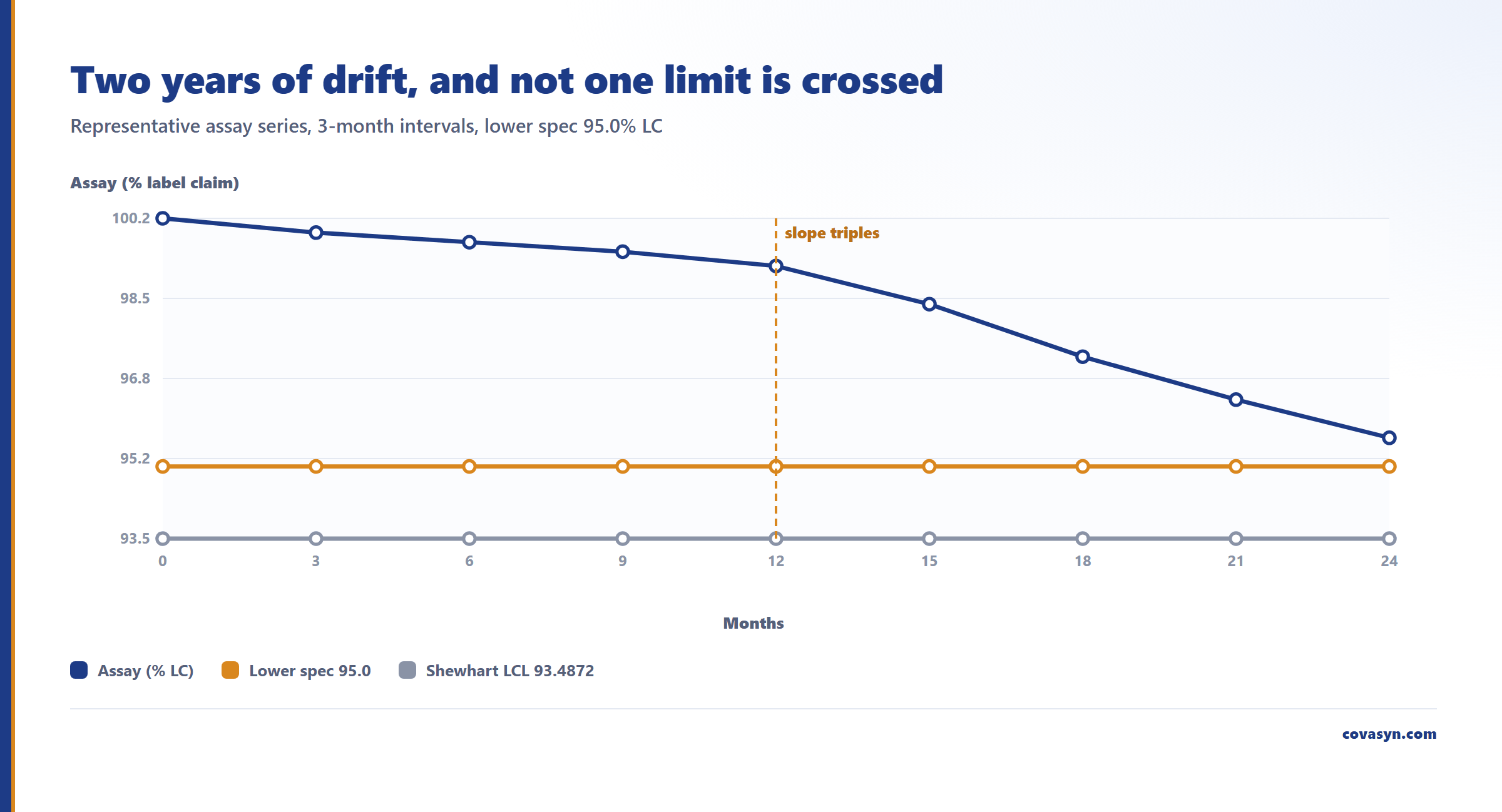
The drift inflates sigma, and the inflated sigma widens the limits that should catch it. The final 95.6% sits just 0.45 above the 95.1470 warning limit. Source: Representative small-molecule stability series analysed with covastab_detect_oos and covastab_control_chart; the mean 98.4667 and LCL 93.4872 are verbatim tool output.

The first five points sit on a shallow slope. From month 12 the slope roughly triples. By eye it is obvious. Here is what the tools returned.

`covastab_detect_oos`

with spec_lower = 95.0: all nine points returned flag: "normal". Zero OOS results across the whole study. The batch is compliant at every single timepoint, and a purely OOS-driven review would close the file with no action.

`covastab_significant_change`

on the same series: has_significant_change: false, max_change_pct: 4.4, spec_violated: false. A 4.4 % loss from baseline, against the ICH 5 % significant-change criterion for assay. Under the threshold, so no formal trigger - but 4.4 % of your 5 % budget is spent, and the last three intervals used most of it.

`covastab_control_chart`

(Shewhart) on the same series: mean 98.4667, UCL 103.4461, LCL 93.4872, warning limits 101.7863 and 95.1470, and ooc_points: []. No out-of-control points. That is correct behaviour, and it shows the blind spot directly: the final value of 95.6 is only 0.45 above the warning limit, because the limits were computed from a series that contains the drift. Drift inflates sigma, sigma widens the limits, and the widened limits swallow the drift.

So three tools, three "no flag", on a series any stability scientist would escalate. Limit-based and shock-based methods are structurally the wrong instrument for slow trend.

Where the real signal is.

Segment the series. Months 0 to 12 lose 1.0 % LC over four intervals. Months 12 to 24 lose 3.6 % over the same four intervals. That change in slope is the finding, and it is what a regression-with-interval or CUSUM approach exists to formalise. On the same representative dataset family, covastab_estimate_shelf returned a shelf life of 28.2 months (R2 0.9989, slope p = 1.3e-8) and covastab_fit_arrhenius returned Ea 107.45 kJ/mol with Q10 4.08 and R2 0.995 - numbers documented in our earlier CovaStab provenance set. A slope that steepens after month 12 breaks the linearity assumption those figures rest on. That is the practical reason OOT matters: it does not just flag a batch, it tells you your shelf-life model is wrong.

The contrast case: a genuine OOS

Second series, same spec, one deliberate excursion at month 18:

100.1, 100.0, 99.9, 100.2, 99.8, 100.0, 93.5, 99.9, 100.1

covastab_detect_oos flagged exactly one point: value 93.5, flag: "OOS", detail "Below lower spec (95.0)". Clean, correct, unambiguous.

covastab_control_chart on the same series returned mean 99.2778, UCL 105.7882, LCL 92.7674, warning limits 103.6180 and 94.9375, with ooc_points: [] again. The 93.5 point sits below the 2-sigma warning limit but above the 3-sigma LCL, because that one outlier inflated the sigma used to build its own limits. Estimate limits from a clean baseline period, not from the series under test.

Honest limits: what these tools did not do

`covastab_detect_oot` returned no flags at all. We called it with method = regression, method = cusum and method = shewhart, on both series above, including the one with a blatant 6.6 percentage-point excursion. Every call returned an empty result list. On this input shape the OOT detector is not usable today, and it is reported to CovaStab engineering. We publish that rather than quietly swap in a number from somewhere else. Use covastab_control_chart and covastab_significant_change plus your own segmented regression until it is fixed.
`covastab_detect_oos` echoes `timepoint: 0` for every row. The flags and values are correct; the timepoint field does not carry the input month. Map results back by row order, not by the returned timepoint.
`covastab_significant_change` appeared to ignore the `initial_value` argument. We passed 100.2; the returned assay_change_pct of 0.2 and max_change_pct of 4.4 are both consistent with a 100.0 baseline. Check the baseline the tool actually used before quoting the percentage.
None of this is a released-batch decision. These are triage signals on numbers you already have. An OOT signal starts an investigation; it does not conclude one, and it is not a substitute for your validated stability protocol, your OOS SOP or a regulatory submission.
Small series. Nine timepoints is a normal stability dataset and a small statistical sample. Control limits from nine points are wide by construction. Trend conclusions firm up when you pool across batches, and pooling itself has to be justified (ICH Q1E poolability testing).

Limit-based and shock-based tests are the wrong instrument for slow drift. covastab_detect_oot returned an empty list for all three methods; the segmented slope is what finds it. Source: Verbatim results from covastab_detect_oos, covastab_significant_change, covastab_control_chart and covastab_detect_oot on the series in this article; the slope comparison is arithmetic on the same nine values.

A practical OOT procedure

1. Fix the method before the data arrives. Write into the protocol which test applies to which parameter, and at what alpha. 2. Build control limits from a clean historical baseline, not from the series you are judging. 3. Run the limit check (covastab_detect_oos) and the trend check separately. One passing does not excuse the other. 4. Segment the series and compare early slope with late slope. A slope change is the most common real OOT finding. 5. Re-fit the shelf-life model after any confirmed trend. If the slope changed, so did the extrapolation behind your expiry date.

Frequently asked questions

What does out of trend (OOT) mean in stability data?

An OOT result is a stability result that is still inside its registered specification but does not match the expected behaviour of the batch or product. It is identified statistically - by regression against historical batches, by a control chart, or by CUSUM - rather than by comparison with a limit. OOT is an early warning that a batch may fail before its expiry date, while every individual result still passes.

What is the difference between OOT and OOS?

OOS means a single result crossed a registered specification limit; it is a direct comparison and needs no statistics. OOT means a pattern across timepoints deviates from expected behaviour while all results remain within specification. OOS triggers a formal investigation and a batch decision. OOT triggers a trend investigation and often a shelf-life model review. A batch can be OOT for years without ever being OOS.

Which statistical method detects out-of-trend stability results best?

It depends on the failure mode. Shewhart control charts detect sudden shocks but miss slow drift, because drift inflates the sigma used to build the limits. CUSUM detects sustained small shifts of about 0.5 to 1 sigma far earlier and is the right choice for gradual degradation. Regression with prediction or tolerance intervals is best for asking whether one batch degrades faster than its siblings.

Can a stability result be out of trend but still in specification?

Yes, and that is the usual case. In our worked example a series falling from 100.2 to 95.6 % label claim against a 95.0 % lower spec returned zero OOS flags from covastab_detect_oos and has_significant_change: false from covastab_significant_change, with a 4.4 % maximum change against the ICH 5 % criterion. Every point passed while the slope tripled after month 12.

Does an OOT result require a formal investigation?

Regulatory guidance does not mandate an OOS-style formal investigation for OOT, but inspectors expect a documented, pre-defined trending procedure and a recorded response when it fires. Practically: define the method and threshold in the protocol before the data exists, document the evaluation, and escalate to a shelf-life or process review when a trend is confirmed across timepoints or batches.

How many timepoints do you need before trend analysis is meaningful?

Control limits and regression intervals from a typical nine-point stability series are wide, so early trends are easy to miss and single points are hard to call. Trend conclusions firm up when you pool several batches, and pooling has to be justified first - ICH Q1E poolability testing checks whether slopes and intercepts are similar enough to combine.