

You fit a quadratic response surface, R squared comes back at 0.9988, and everything looks finished. Then the diagnostics panel flags a normality test at p = 0.036 and points at run 9. The question is not whether the flag is real. The question is whether it means your model is wrong, or whether it means your design is doing exactly what a central composite design is supposed to do.
What residual diagnostics are actually for
A response surface model gives you coefficients, p-values and an R squared. None of those tell you whether the *assumptions behind* those numbers held. Residual diagnostics do. They are the model auditing itself.
Three checks carry almost all of the weight:
- Shapiro-Wilk asks whether the residuals look normally distributed. Normality is what your confidence intervals, prediction intervals and term p-values are built on.
- Cook's distance asks how much the whole fitted surface would move if you deleted one run. It is influence, not error.
- Leverage (the hat-matrix diagonal) asks how far a run sits from the centre of the design in factor space. It is a property of the *design*, not of the data you measured.
Confusing the last two is the most common mistake we see. High leverage is not a defect. It is the reason axial points exist.
A worked example on a real central composite design
The numbers below come from the same 18-run central composite design (8 factorial, 6 axial, 4 centre) used in our RSM design-space work: a 3-factor catalytic step (temperature, catalyst loading, time), fitted as a quadratic at R squared 0.9988 (adjusted 0.9974), then audited with CovaSyn's residual diagnostics.
Caveat up front, because it matters for how you read these figures: the CCD itself is a genuine design and every statistic quoted is genuinely computed, but the per-run yields were simulated from a quadratic surface with added noise to stand in for lab measurements. Treat the *behaviour* of the diagnostics as the lesson, not the specific yield values.
| Diagnostic | Result | Conventional cutoff | Read |
|---|---|---|---|
| Shapiro-Wilk W | 0.888, p = 0.036 | p < 0.05 rejects normality | Normality rejected |
| Max Cook's distance | 0.277 at run 9 | 4/n = 0.222 (sensitive); 1.0 (influential) | Flagged, not influential |
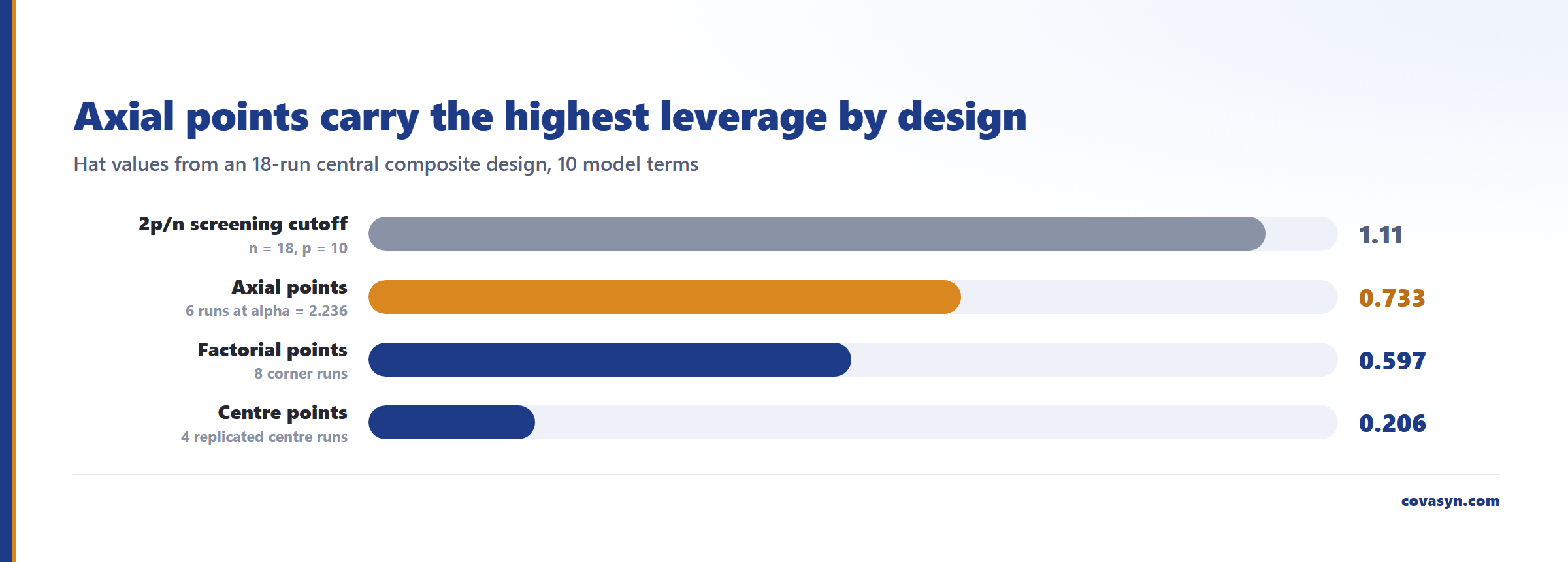
| Leverage, centre points | 0.206 | 2p/n = 1.11 | Low, as designed |
| Leverage, factorial points | 0.597 | 2p/n = 1.11 | Normal |
| Leverage, axial points | 0.733 | 2p/n = 1.11 | Highest, as designed |
n = 18 runs, p = 10 model terms (intercept, 3 linear, 3 two-factor interactions, 3 quadratic).
Sanity check you can do yourself
Leverages in an ordinary least squares fit must sum to the number of estimated parameters. Here: 4 x 0.206 + 8 x 0.597 + 6 x 0.733 = 9.998, which is 10 to rounding. That is the number of terms in the quadratic model. If your software returns leverages that do not sum to p, something upstream is broken: a duplicated row, a dropped term, a rank-deficient design. It is a 10-second check and it catches real problems.
Why the axial points show the highest leverage, and why that is fine
In this central composite design the axial (star) points sit at alpha = 2.236 in coded units, further from the design centre than any factorial corner. Leverage rises with distance from the centroid, so axial points *must* have the highest hat values. That is not a bug in the experiment. Those points are the only runs that let you estimate pure quadratic curvature at all. Remove them and the model cannot see curvature, which is the whole reason you ran a CCD instead of a factorial.
So when a diagnostics panel highlights an axial run, the correct first reaction is: expected. The design put that point out there on purpose, and the fit is leaning on it on purpose.
At 0.733 the axial leverage here is nowhere near the usual 2p/n = 1.11 screening cutoff. Nothing in this design is an outlier in factor space.
How to read Cook's distance of 0.277
Cook's D combines leverage with residual size. Run 9 came back at 0.277, the largest in the set.
Two cutoffs are in common use, and they disagree on purpose:
- 4/n, here 4/18 = 0.222. A deliberately sensitive screen. 0.277 exceeds it, which is why the run gets flagged.
- D > 1. The classical "this run is genuinely influential" threshold. 0.277 is nowhere near it.
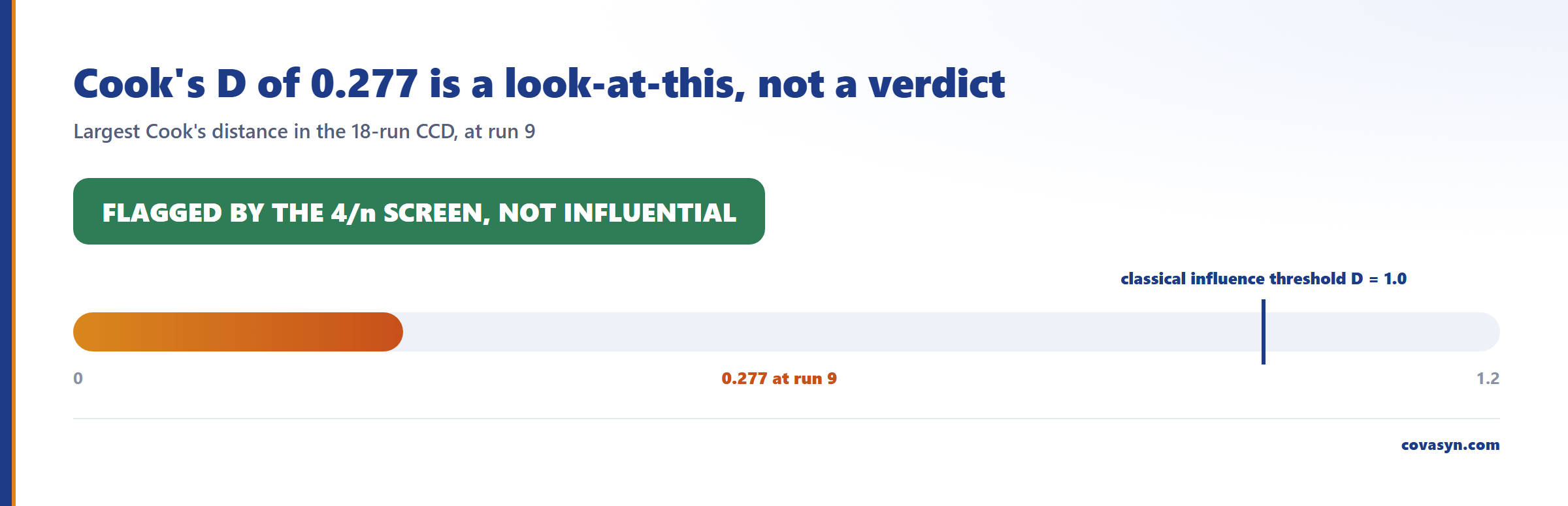
The honest reading: run 9 pulls the surface more than its neighbours, but deleting it would not meaningfully move the fitted model. It is a look-at-this, not a stop-the-press. What you do with it is go back to the batch record for that run: check whether the temperature actually held, whether the sample was pulled on time, whether the assay was re-injected. If the run is clean, keep it. Never delete a point because a statistic flagged it and the record says nothing was wrong.
How to read Shapiro-Wilk W = 0.888, p = 0.036
The test rejects normality. Before you re-transform your response, three things are worth knowing.
First, n = 18. Shapiro-Wilk on 18 residuals has low power against real departures and is noisy against harmless ones. A p just under 0.05 on 18 points is weak evidence, not a verdict.
Second, when R squared is 0.9988 the residuals are tiny. What is left is close to pure measurement noise plus the small systematic bit the quadratic form cannot absorb. A single moderately sized residual can drag W down without any of the residuals being large in units you care about.
Third, and most usefully: read the normality flag *together* with the Cook's D flag. Both point at the same region of the design. That is a consistent story: one run sits slightly off the surface, it is the same run inflating Cook's D, and it is the same run that makes the residual set look non-normal. One explanation, two symptoms. That is much more informative than either number alone.
Practical response, in order: 1. Check the batch record for the flagged run. 2. Refit without it and compare coefficients and the optimum location. If nothing moves, the flag is cosmetic. 3. Only if the residual spread grows with the fitted value should you consider a variance-stabilising transform (log, square root) or weighted least squares. 4. If curvature is still visible in the residuals-versus-fitted plot, the model form is wrong, not the data. Add terms or shrink the modelled region.
What these diagnostics do not tell you
- They cannot validate the model outside the design region. Every statistic here is conditional on the ranges you actually ran. Extrapolation is unprotected.
- They cannot tell you a flagged run is a bad measurement. Only the batch record and the analyst can. Statistics identify candidates for review.
- Normality of residuals is not normality of the response. Do not transform the response because the raw yields look skewed.
- A clean diagnostic panel is not a validated process. It says the regression assumptions are defensible. It says nothing about robustness, scale-up or whether your assay is fit for purpose.
- These are decision-support outputs, not a filing. They belong in your development report as supporting evidence, alongside wet-lab confirmation runs.
Frequently asked questions
What is a good Cook's distance threshold for a designed experiment?
Two thresholds are standard. The sensitive screen is 4/n, so 0.222 for an 18-run design. The classical influence threshold is D greater than 1. A value between them, such as the 0.277 at run 9 in the worked example, means the run deserves a look at the batch record but would not meaningfully change the fitted surface if removed. Never delete a run on the statistic alone.
Why do axial points in a central composite design have high leverage?
Axial or star points sit further from the design centre than any factorial corner, at a coded alpha greater than 1, here 2.236. Leverage grows with distance from the centroid, so axial runs always carry the highest hat values. In a real 18-run CCD that was 0.733 for axial points versus 0.206 for centre points. This is by design: axial runs are what allow the pure quadratic terms to be estimated at all.
Does a failed Shapiro-Wilk test invalidate my response surface model?
Not on its own. With small designed experiments the test has limited power and a marginal p-value carries little weight. A real fit in the worked example returned W = 0.888 at p = 0.036 on 18 residuals with R squared 0.9988. The practical step is to check whether the same run also drives Cook's distance, inspect residuals versus fitted values for structure, and only transform the response if the variance clearly scales with the fitted value.
How many residuals do you need for Shapiro-Wilk to be meaningful?
Shapiro-Wilk is usable from about n = 7 but has weak power below roughly n = 30. Typical DoE sizes, 12 to 20 runs, sit squarely in the low-power region. That means a pass is weak reassurance and a marginal fail is weak evidence of a problem. Use the test as one input alongside residual plots and Cook's distance rather than as a gate.
What is the difference between leverage and influence?
Leverage is a property of the design matrix alone: how far a run sits from the centre of factor space. It is known before you measure anything. Influence, measured by Cook's distance, combines leverage with how badly that run is fitted. A high-leverage run that lands exactly on the surface has almost no influence. Influence only appears when an unusual factor setting also produces an unexpected response.
Can residual diagnostics detect a wrong model form?
Partly. Systematic curvature in a residuals-versus-fitted plot indicates missing terms, and lack-of-fit tests against replicate centre points test this directly. But Shapiro-Wilk and Cook's distance alone will not distinguish a missing interaction term from measurement noise. Always inspect the residual plots, and use replicated centre points so a formal lack-of-fit test is available.
Related reading
Evaluation for this topic
We evaluate this for your lab.
- Design of Experiments, RSM, templates.