CovaSolv benchmarked: predicting solubility at R² 0.92, and why the honest number is the more important one
CovaSolv predicts logS at R² 0.92 and RMSE 0.64, on 5,315 unseen molecular scaffolds. 78 % of predictions sit within 0.5 log units of the measured value. How close that is to the physical noise floor, honestly explained.
Oliver Kraft
CovaSyn

Key takeaways
- CovaSolv predicts solubility (log S) at R² 0.92, RMSE 0.64 log; 78 % of all predictions land within 0.5 log units of the measured value.
- That number comes from a scaffold holdout: tested on 5,315 molecular cores the model has never seen, not a flattering random split.
- It sits practically at the physical noise floor: experimental solubility reproducibility between labs is roughly 0.6 log.
- CovaSolv clearly beats the classical ESOL equation (RMSE 0.69 vs. 0.96; R² 0.91 vs. 0.55) and is competitive to better than current ML models.
- Every prediction comes with a calibrated uncertainty interval and an applicability-domain flag, the model tells you when it is extrapolating.
The number first
Solubility is one of the earliest and most consequential properties in drug development. It governs bioavailability, formulability, and the solvent choice in every crystallization and purification step. And it is notoriously hard to predict.
CovaSolv, the solubility module of the CovaSyn platform, predicts the decadic logarithm of solubility (log S, in mol/L) with the following accuracy:
- R² = 0.920
- RMSE = 0.636 log
- MAE = 0.371 log
- 78.0 % of predictions within 0.5 log
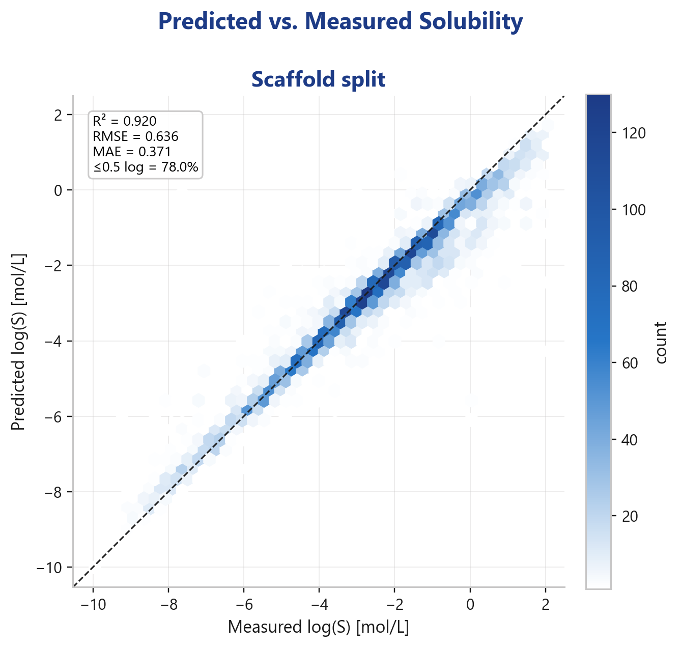
The parity plot hugs the diagonal across more than ten log units. Crucially: this is the deployed production model evaluated on held-out data, not a training-time metric that you score against yourself.
But how honest is that number?
This is where it gets interesting, because solubility benchmarks live or die by their test methodology.
The easy path is a random split: shuffle all molecules, take 80 % for training and 20 % for testing. The problem: closely related analogues of the same molecular core then end up in both buckets. The model has practically peeked at the test set during training and sees old friends at evaluation time. The numbers look great, and collapse the moment a genuinely new scaffold turns up in real research.
We therefore test via scaffold holdout: entire molecular cores are removed from training and only shown at test time. The model has to generalize across structurally new classes, exactly the situation medicinal chemistry faces every day. It is the hard, honest metric, and that is where CovaSolv earns its R² 0.92.
In short: we report the difficult number, not the easy one.
CovaSolv operates at the physical noise floor
The second question is: how much better can a model even get?
The answer is physically bounded. Measure the same compound in different labs and the results scatter: the published inter-lab reproducibility of experimental solubility sits at roughly 0.6 log units. That is the baseline noise of the real data itself, no model can be more consistent than the data it is trained and measured against.
CovaSolv's RMSE of 0.64 to 0.69 log thus sits practically on that noise floor. On broad, diverse real-world data, more is barely measurable, the remaining difference vanishes into experimental noise. That is a strong claim, and it is honest: getting closer is almost physically impossible.
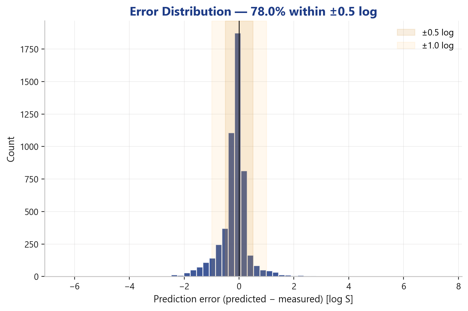
The error distribution shows it cleanly: a sharp, symmetric peak around zero, no systematic bias, thinly trailing tails. The bulk of predictions sits inside the ±0.5 log band, the vast remainder inside ±1.0 log.
Compared to the literature
A single number says little, it needs context. The established reference point for aqueous solubility is the ESOL equation (Delaney 2004), still a widely cited baseline.
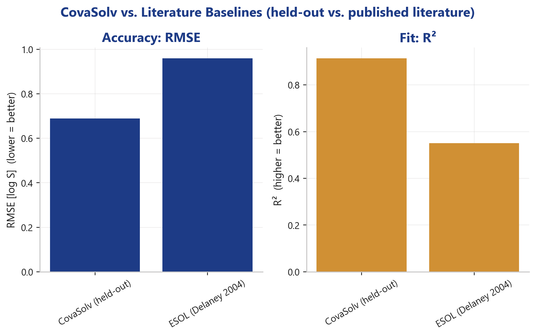
- CovaSolv (held-out, aqueous): RMSE 0.69 · R² 0.91
- ESOL (Delaney 2004): RMSE 0.96 · R² 0.55
CovaSolv significantly lowers the error and nearly doubles the explained variance. For context against newer ML approaches (published values): a 2025 LightGBM model sits at RMSE ≈ 0.85, a SolTranNet transformer at ≈ 1.46, and the average Solubility Challenge participant at ≈ 1.14.
A fairness note that belongs here:
those literature values come from different test sets. A direct head-to-head comparison therefore tends to overstate the gap, anyone using a different test set is measuring a different task. We say so openly rather than hide it. And for the ESOL comparison we deliberately use the aqueous held-out subset of CovaSolv (RMSE 0.69), because ESOL is a pure water-solubility model, a mixed-solvent comparison would tilt unfairly in CovaSolv's favor.
The model knows its limits
A point estimate without context is dangerous in research. The actually valuable property of a prediction model is not only what it says, but how confident it is.
CovaSolv ships two trust layers:
- Applicability-domain flag. The model itself flags when a query lies outside the chemical space it can reliably cover, for very large or structurally novel molecules, for example. Instead of a confident-sounding but unsupported number, you get an honest warning.
- Conformal prediction intervals. Every prediction comes with a calibrated uncertainty interval, no blind point estimate but a quantified range that a scientist can actually use for risk-weighted decisions.
The message: a model you can trust because it tells you when to trust it.
Verifiable on known drugs
Trust comes from verifiability. So here are the predictions for common, well-measured drugs against their experimental values, anyone can cross-check:
- Aspirin: predicted −1.61 · experimental −1.72 · absolute error 0.11
- Paracetamol: predicted −1.14 · experimental −1.03 · error 0.11
- Benzoic acid: predicted −1.32 · experimental −1.55 · error 0.23
- Lidocaine: predicted −1.94 · experimental −1.70 · error 0.24
- Ibuprofen: predicted −3.94 · experimental −3.62 · error 0.32
- Caffeine: predicted −0.98 · experimental −0.60 · error 0.38
- Carbamazepine: predicted −3.50 · experimental −3.01 · error 0.49
- Salicylic acid: predicted −1.37 · experimental −1.94 · error 0.57
- Naproxen: predicted −3.54 · experimental −4.21 · error 0.67
Most errors sit well below 0.5 log, and even the larger ones are within the order of magnitude of experimental noise.
Holds up on modern, complex molecules
Classical models were trained on simple, small molecules and fail in today's pharma reality. CovaSolv delivers predictions, with uncertainty and AD flag, into current, difficult structures:
- Osimertinib: −3.24 log S · 90 % interval [−3.4; −3.0] · in domain
- Nirmatrelvir: −2.58 · [−3.1; −2.0] · in domain
- Sotorasib: −4.25 · [−4.5; −4.0] · in domain
- Exatecan: −3.29 · [−3.3; −3.2] · in domain
- Deruxtecan: −2.43 · [−3.5; −1.4] · in domain
- MMAE: −3.14 · [−3.4; −2.8] · in domain
Notably: even ADC payloads like Exatecan, Deruxtecan and MMAE, structures where simpler models fail in droves, stay inside the applicability domain. Where the interval widens (Deruxtecan), the model communicates the larger uncertainty honestly instead of hiding it.
More than a number, practical value
A good log-S number is a means to an end. What matters in the lab and in process development is what you do with it. CovaSolv answers the questions that actually come up in the workflow.
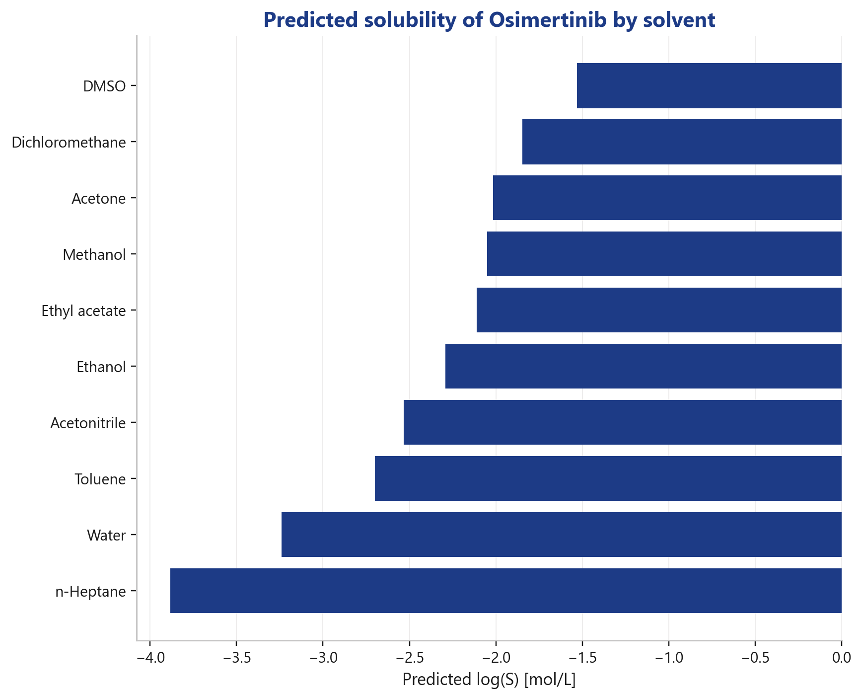
Which solvent dissolves my compound best?
A solvent ranking across common process solvents, for Osimertinib the predicted solubility ranges from DMSO (best) down to n-heptane (worst).
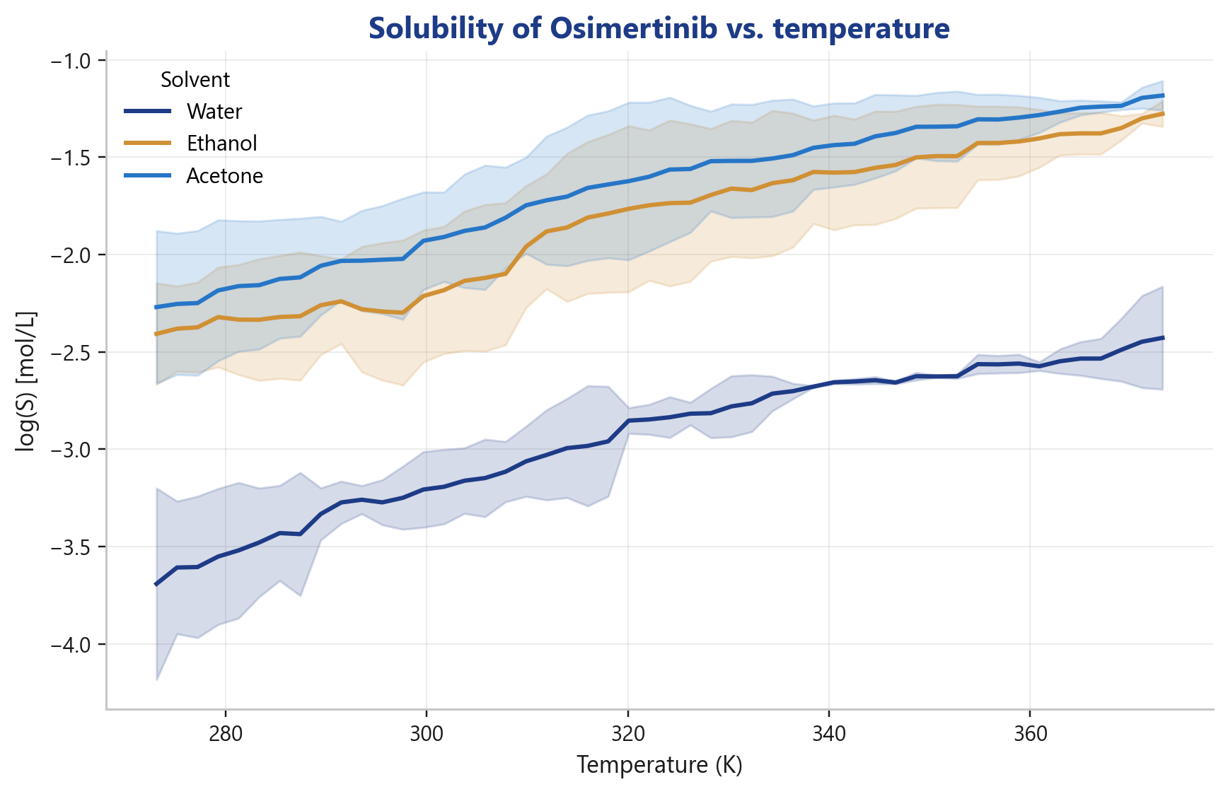
How does solubility vary with temperature?
Temperature curves including uncertainty bands form the basis for designing cooling crystallizations.
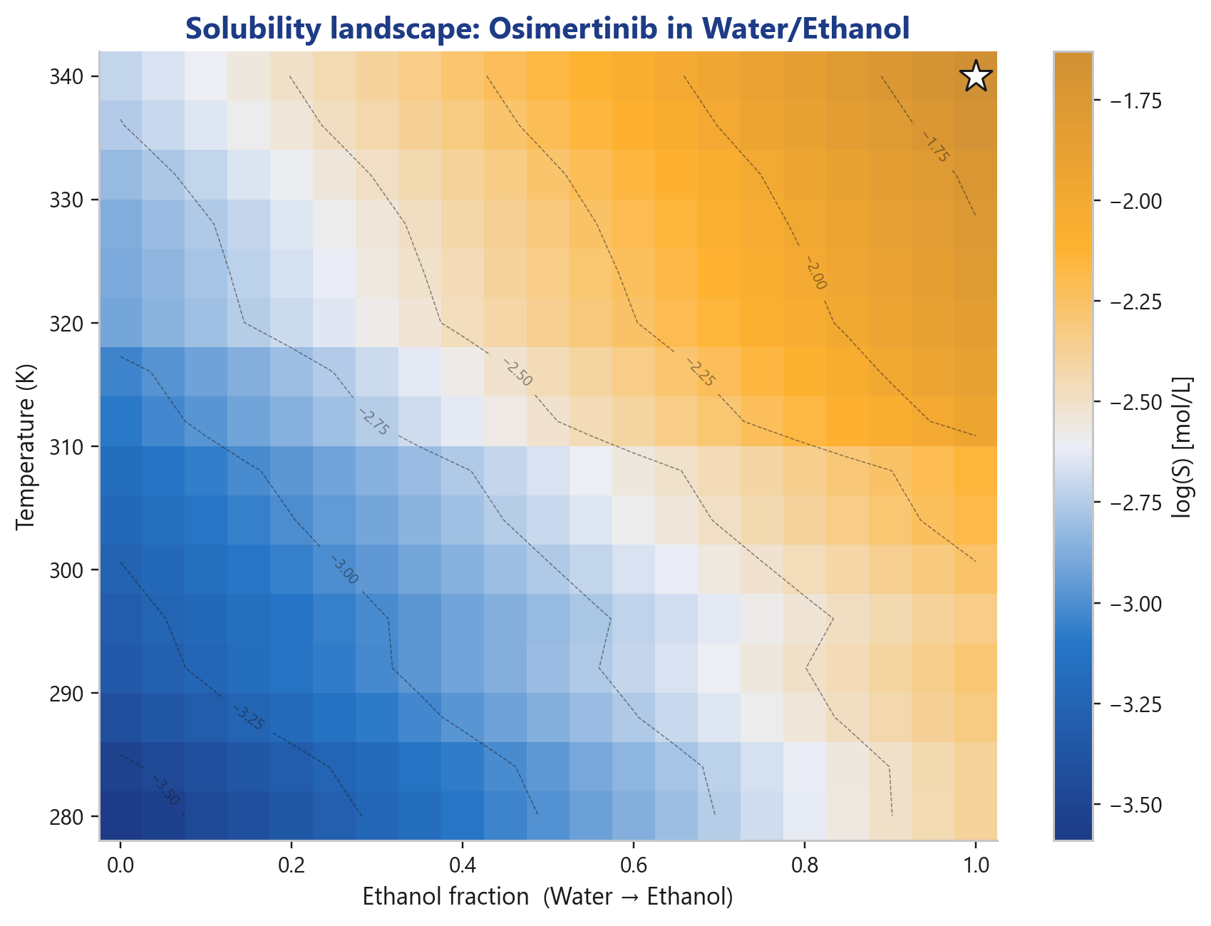
And in a solvent mixture?
The solubility landscape across temperature × ethanol fraction shows the optimum at a glance, the starting point for anti-solvent and cooling-crystallization strategies in process development.
That is the transition from "interesting prediction" to "usable process decision", and that is exactly where the value lives in CMC and pre-formulation work.
The data basis
Solid numbers need solid data. CovaSolv is trained on 95,633 solubility measurements (from BigSolDB v2.0 and OChem), uses 339 selected molecular features, and is built on an XGBoost/LightGBM ensemble. The architecture is deliberately classical and robust rather than experimental, because reproducibility in regulated workflows matters more than novelty for its own sake.
Why solubility prediction is hard, and why naïve benchmarks mislead
To close, the honest context that puts these numbers in perspective.
Solubility is hard for three reasons. First, experimental noise (the ~0.6 log mentioned above). Second, the difference between apparent and intrinsic solubility, measured values depend on solid-state form, polymorphism, and experimental conditions. Third, ionization: pH and pKa shift apparent solubility by orders of magnitude.
And the most important reason to be cautious with benchmark comparisons: training overlap (leakage). Public challenge sets partially overlap with the large training databases. A model that has already seen part of the "test" set during training reports brilliant but meaningless numbers. That is precisely why we test by scaffold holdout and call out test-set differences explicitly.
We publish this openly because a credible number is worth more than an impressive one. The full methodology and all raw metrics sit at covasyn.com/benchmark.
See it for yourself
The free tier lets you attach CovaSolv directly to your AI agent, Claude, ChatGPT, Cursor or Copilot, and query log-S predictions, solvent rankings and temperature curves for your own structures. 100 credits per week. → See CovaSyn MCP
FAQ
How accurate is AI-based solubility prediction?
CovaSolv achieves R² 0.92 and RMSE 0.64 log on a scaffold holdout of 5,315 unseen molecular cores; 78 % of predictions sit within 0.5 log. That is near the physical noise floor of roughly 0.6 log inter-lab reproducibility.
What is a good RMSE for a solubility model?
Because experimental solubility scatters by ~0.6 log across labs, an RMSE in the 0.6 to 0.7 log range is practically the ceiling on diverse real data. CovaSolv sits there at 0.64 to 0.69.
What is the difference between scaffold split and random split?
A random split overestimates accuracy because related molecules end up in training and test. A scaffold split holds back entire cores and measures real generalization to new structural classes. CovaSolv reports the scaffold number.
Does CovaSolv beat the ESOL equation?
Yes. On the aqueous held-out subset CovaSolv hits RMSE 0.69 and R² 0.91 vs. 0.96 and 0.55 for ESOL (Delaney 2004).
How do I know I can trust a prediction?
Every CovaSolv prediction comes with a calibrated conformal interval and an applicability-domain flag that signals when the model is extrapolating.
Methodology and data
Model: CovaSolv (XGBoost/LightGBM ensemble, 339 features). Training: 95,633 measurements from BigSolDB v2.0 and OChem. Evaluation: scaffold holdout, 5,315 held-out compounds (R² 0.920 / RMSE 0.636 / MAE 0.371 / 78.0 % ≤ 0.5 log); aqueous held-out subset for the ESOL comparison (RMSE 0.689 / R² 0.914 / 76.4 % ≤ 0.5 log). Literature values (ESOL, LightGBM 2025, SolTranNet, Solubility Challenge) come from published, different test sets and are to be read as order of magnitude only. Data snapshot: 2026-05-21.
CovaSyn MCP
Scientific tools in your AI workflow.
130+ functions for pharma, biotech and chemistry. Free tier instantly active.